smoothEMr

The goal of smoothEMr is to efficiently implement the SmoothEM algorithm for various GMRF priors, using different initialization strategies.

Installation

You can install the development version of smoothEMr like so:

pak::pak("AgueroZZ/smoothEMr")

Example

This is a basic example which shows you how to solve a common problem:

library(smoothEMr)

We will simulate some data from a spiral embedded in 2D space, and then fit a smoothEM model to it.

simulate_swiss_roll_1d_2d <- function(n = 800,
                                     t_range = c(1.5 * pi, 6 * pi),
                                     sigma = 0.15,     # can be scalar or length-2
                                     seed = 1) {
  stopifnot(length(t_range) == 2)
  stopifnot(length(sigma) == 1 || length(sigma) == 2)

  set.seed(seed)

  # 1D parameter
  t <- runif(n, min = t_range[1], max = t_range[2])

  # true 2D "swiss roll" (spiral)
  x_true <- t * cos(t)
  y_true <- t * sin(t)

  # noise
  if (length(sigma) == 1) sigma <- rep(sigma, 2)
  x_obs <- x_true + rnorm(n, 0, sigma[1])
  y_obs <- y_true + rnorm(n, 0, sigma[2])

  list(
    t = t,
    truth = data.frame(x = x_true, y = y_true),
    obs   = data.frame(x = x_obs,  y = y_obs)
  )
}

sim <- simulate_swiss_roll_1d_2d(n = 1500, sigma = 0.2, seed = 123)

plot(sim$obs$x, sim$obs$y, pch = 16, cex = 0.35, col = "grey80",
     xlab = "x", ylab = "y", main = "Noisy 2D swiss-roll (spiral)")
pal <- colorRampPalette(c("navy", "cyan", "yellow", "red"))(256)
t_scaled <- (sim$t - min(sim$t)) / (max(sim$t) - min(sim$t))  # in [0,1]
col_t <- pal[pmax(1, pmin(256, 1 + floor(255 * t_scaled)))]
points(sim$truth$x, sim$truth$y, pch = 16, cex = 0.25, col = col_t)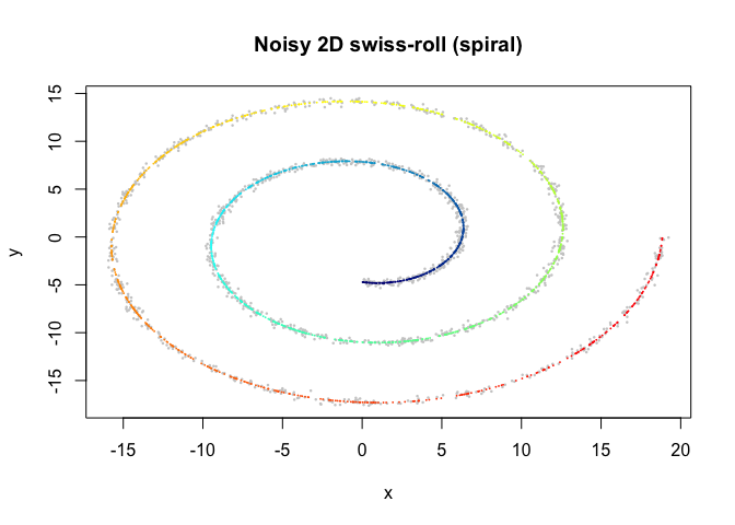

Now we fit a smoothEM model to the noisy observations.

# initialize using tSNE
fit <- initialize_smoothEM(X = as.matrix(sim$obs), method = "tSNE", rw_q = 2)

# run 10 iterations of smoothEM
fit <- fit |>
  do_smoothEM(iter = 10)

# plot results
plot(fit)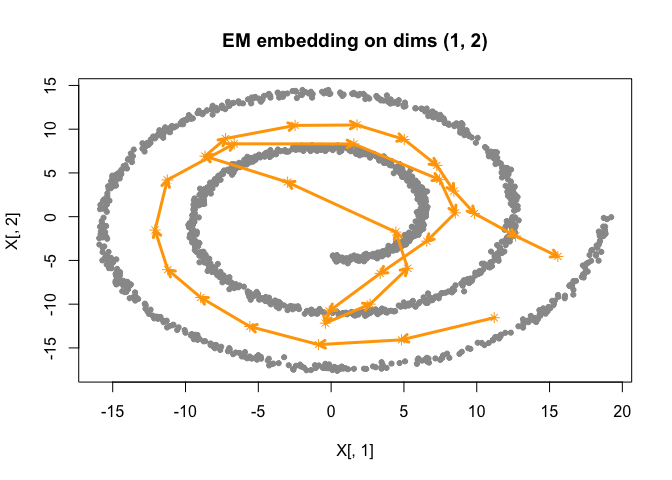

plot(fit, plot_type = "elbo")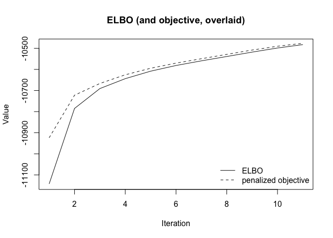

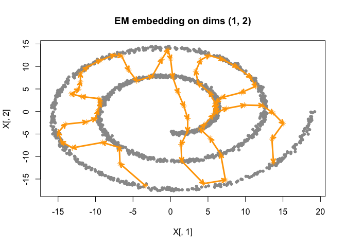
We could also try other initialization methods, such as PCA or Fiedler vector initialization.

fit_pca <- initialize_smoothEM(X = as.matrix(sim$obs), method = "PCA", rw_q = 2) |>
  do_smoothEM(iter = 50)
plot(fit_pca)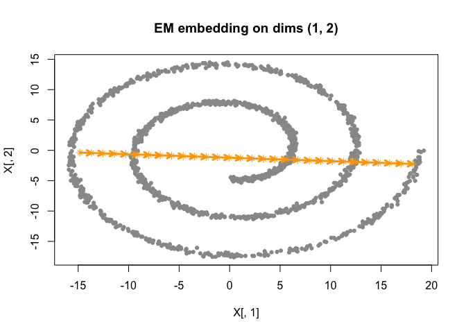

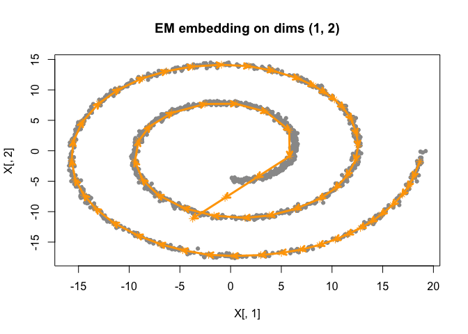
fit_fiedler <- initialize_smoothEM(X = as.matrix(sim$obs), method = "fiedler", rw_q = 2) |>
  do_smoothEM(iter = 50)
plot(fit_fiedler)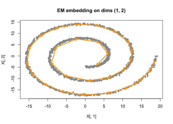

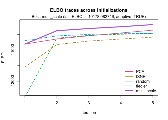
To automatically select the best initialization method, we can use:

best <- optimize_initial(
  as.matrix(sim$obs),
  num_iter = 5,
  num_cores = 6,
  m_max = 6,
  two_panel = FALSE,
  plot = TRUE
)

plot(best, plot_type = "scatterplot", dims = c(1,2))

best_fit <- best |>
  do_smoothEM(iter = 50)

plot(best_fit)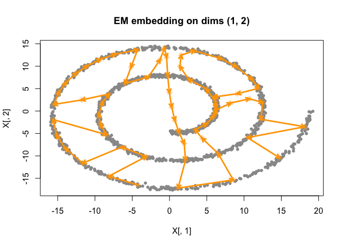

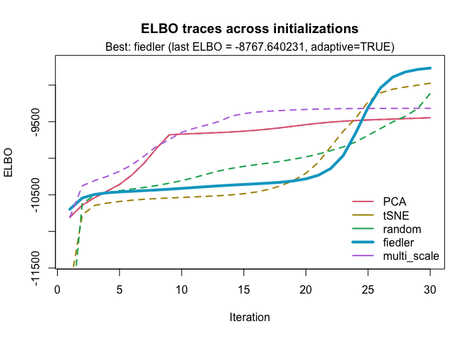
If we choose a different choice of num_iter, we could end up with a different optimal initialization:

best_2 <- optimize_initial(
  as.matrix(sim$obs),
  num_iter = 30,
  num_cores = 6,
  m_max = 6,
  two_panel = FALSE,
  plot = TRUE
)

plot(best_2, plot_type = "scatterplot", dims = c(1,2))