Intro to smoothEMr

Model overview

smoothEMr fits a Gaussian mixture model with a structured (smoothness) prior on the component means. Let $X_i \in \mathbb{R}^d$ be the observed vector for $i = 1,\dots,n$, and let $z_i \in \{1,\dots,K\}$ be the latent component label. The observation model is

$$X_i \mid z_i = k \sim N(\mu_k, \Sigma), \qquad \Pr(z_i = k) = \pi_k .$$

To encourage ordered / smooth transitions across components $k=1,\dots,K$, we place a multivariate normal prior on the stacked mean vector $U = (\mu_1^\top, \dots, \mu_K^\top)^\top$:

$$U \sim N(0, Q_\lambda^{-1}),$$

where the precision matrix $Q_\lambda$ encodes the desired structure across components. For computational efficiency, we require $Q_\lambda$ to be sparse so the prior is a GMRF (Gaussian Markov random field). Many common GMRF priors can be interpreted as discrete analogues of continuous GP priors. Equivalently, the M-step solves a penalized optimization problem with quadratic penalty $\tfrac{1}{2} U^\top Q_\lambda U$.

The default choice in smoothEMr is a $q$-th order random-walk (RW) prior, with

$$Q_\lambda = \lambda Q_{\mathrm{rw}q},$$

where $Q_{\mathrm{rw}q}$ is the precision matrix induced by $q$-th order discrete differences. Larger $\lambda$ enforces stronger smoothness across neighboring components.

Equivalently, letting $\mu_{\cdot,j} = (\mu_{1,j},\dots,\mu_{K,j})^\top \in \mathbb{R}^K$, the RW2 penalty can be written as $$\sum_{k=3}^K \big(\mu_{k,j} - 2\mu_{k-1,j} + \mu_{k-2,j}\big)^2 \;=\; \mu_{\cdot,j}^\top Q_{\mathrm{rw}2}\,\mu_{\cdot,j}, \qquad Q_{\mathrm{rw}2} = D_2^\top D_2,$$ where $D_2 \in \mathbb{R}^{(K-2)\times K}$ is the second-difference matrix with rows $(0,\dots,0,\,1,\,-2,\,1,\,0,\dots,0)$.

By default, smoothEMr assumes $\Sigma$ is diagonal and shared across components (homoskedasticity), but the framework can be extended to accommodate heteroskedasticity or other covariance structures.

Algorithm overview (smooth-EM)

Fix a smoothing strength $\lambda$ and a sparse precision matrix $Q_\lambda = \lambda Q_{\mathrm{rw}q}$. Let $U = (\mu_1^\top,\dots,\mu_K^\top)^\top$ stack all component means. We seek a MAP estimate by maximizing the log-posterior (up to an additive constant) over $(\pi,U,\Sigma)$:

$$J(\pi,U,\Sigma;\lambda) = \sum_{i=1}^n \log\!\Big(\sum_{k=1}^K \pi_k\, p(X_i \mid \mu_k,\Sigma)\Big) \;-\; \tfrac{1}{2} U^\top Q_\lambda U \;+\; \text{const}(\lambda),$$ where $\text{const}(\lambda)$ collects terms that do not depend on $(\pi,U,\Sigma)$.

The smooth-EM algorithm performs coordinate ascent on an ELBO (evidence lower bound) $\mathrm{ELBO}(\Gamma,\pi,U,\Sigma;\lambda)$ of the form $$\mathrm{ELBO}(\Gamma,\pi,U,\Sigma;\lambda) = \sum_{i=1}^n \sum_{k=1}^K \gamma_{ik} \Big\{ \log \pi_k + \log p(X_i \mid \mu_k,\Sigma) \Big\} \;+\; H(\Gamma) \;-\; \tfrac{1}{2} U^\top Q_\lambda U \;+\; \text{const}(\lambda),$$ where $H(\Gamma) = -\sum_{i,k}\gamma_{ik}\log\gamma_{ik}$ is the entropy term.

Relationship between ELBO and the objective. For any $\Gamma$, $$J(\pi,U,\Sigma;\lambda) \;\ge\; \mathrm{ELBO}(\Gamma,\pi,U,\Sigma;\lambda),$$ and equality holds when $\gamma_{ik} = \Pr(z_i=k \mid X_i,\pi,U,\Sigma)$ (i.e., $\Gamma$ equals the posterior responsibilities). Thus, maximizing the ELBO provides a monotone lower-bound ascent procedure for the MAP objective $J$.

Given current parameter values, each iteration alternates:

1. E-step (update $\Gamma$): $$\gamma_{ik} \propto \pi_k\, p(X_i \mid \mu_k,\Sigma), \quad \text{normalized over } k=1,\dots,K.$$

2. M-step (update $\pi,U,\Sigma$): update $\pi$ and $\Sigma$ in closed form given $\Gamma$, and update $U$ by maximizing $$U \leftarrow \arg\max_U \Big\{ \sum_{i,k} \gamma_{ik}\log p(X_i \mid \mu_k,\Sigma) \;-\; \tfrac{1}{2} U^\top Q_\lambda U \Big\}.$$

With $\lambda$ fixed, the ELBO is non-decreasing over iterations; moreover, because each E-step makes the bound tight at the current parameters, the MAP objective $J$ is also non-decreasing.

A simple 2D example

We simulate data from a spiral (swiss-roll) embedded in 2D space, then fit a smoothEM model.

sim <- simulate_swiss_roll_1d_2d(n = 1500, sigma = 0.2, seed = 123)

plot(sim$obs$x, sim$obs$y, pch = 16, cex = 0.35, col = "grey80",
     xlab = "x", ylab = "y", main = "Noisy 2D swiss-roll (spiral)")

pal <- colorRampPalette(c("navy", "cyan", "yellow", "red"))(256)
t_scaled <- (sim$t - min(sim$t)) / (max(sim$t) - min(sim$t))  # in [0,1]
col_t <- pal[pmax(1, pmin(256, 1 + floor(255 * t_scaled)))]
points(sim$truth$x, sim$truth$y, pch = 16, cex = 0.25, col = col_t)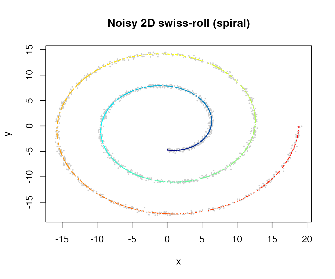

To fit the model, we first initialize the smoothEM algorithm using a given initialization method. Here, we use fiedler initialization and fix the smoothing parameter lambda to 10.

set.seed(123)
fit <- initialize_csmoothEM(
  X = as.matrix(sim$obs),
  method = "fiedler",
  adaptive = FALSE,
  k = 15,
  K = 100,
  lambda = 10
)
fit
#> Fitted csmoothEM object with RW(2) prior along K = 100
#> -----
#>   n = 1500, d = 2, modelName = homoskedastic
#>   iter = 1; init_method = fiedler; adaptive = none;
#>   lambda_vec: range=[10, 10], mean=10, relative = TRUE
#>   ELBO last = -10472.720320; penLogLik last = -10383.239352; ML/C last = -10472.704642

The key function do_csmoothEM() runs smooth-EM updates for a given number of iterations.

fit <- fit |>
  do_csmoothEM(iter = 1)

plot(fit)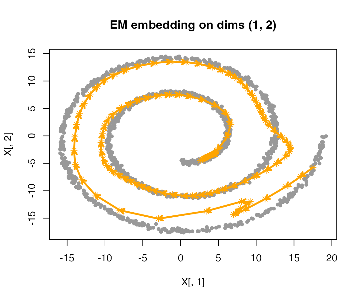

We can also inspect ELBO values over iterations:

plot(fit, plot_type = "elbo")

Adaptive estimation of the smoothing parameter $\lambda$

Optionally, smoothEMr can update $\lambda$ during the EM iterations. Unlike the MAP updates performed when $\lambda$ is fixed, here we aim to optimize the marginal likelihood $$\ell(\lambda)=\log p(X\mid \eta,\lambda)=\log\int p(X\mid \mu,\eta)\,p(\mu\mid \lambda)\,d\mu .$$

The marginal likelihood is generally intractable. Using the ELBO as a surrogate for $\log p(X\mid \mu,\eta)$ yields an approximate marginal likelihood $$\widetilde{\ell}(\lambda) =\log\int \exp\!\big(\mathrm{ELBO}(q;\mu,\eta)\big)\,p(\mu\mid \lambda)\,d\mu .$$

Because the ELBO is (locally) quadratic in $\mu$ and the prior $p(\mu\mid \lambda)$ is Gaussian, we can further obtain a closed-form Laplace approximation. Let $$\widehat{\mu} =\arg\max_{\mu}\Big\{\mathrm{ELBO}(q;\mu,\eta)+\log p(\mu\mid \lambda)\Big\}, \qquad H=-\nabla_\mu^2\!\Big[\mathrm{ELBO}(q;\mu,\eta)+\log p(\mu\mid \lambda)\Big]\Big|_{\mu=\widehat{\mu}} .$$ Then the collapsed objective is $$C(q;\eta,\lambda) =\mathrm{ELBO}(q;\widehat{\mu},\eta)+\log p(\widehat{\mu}\mid \lambda) +\frac{K}{2}\log(2\pi)-\frac{1}{2}\log|H|.$$

To implement adaptive estimation of $\lambda$, we just need to use adaptive = "ml" in the initialization step.

set.seed(123)
fit_ml <- initialize_csmoothEM(
  X = as.matrix(sim$obs),
  method = "fiedler",
  adaptive = "ml"
)
fit_ml
#> Fitted csmoothEM object with RW(2) prior along K = 50
#> -----
#>   n = 1500, d = 2, modelName = homoskedastic
#>   iter = 1; init_method = fiedler; adaptive = ml;
#>   lambda_vec: range=[1.16, 1.39], mean=1.28, relative = TRUE
#>   ELBO last = -10548.204455; penLogLik last = -10500.506958; ML/C last = -10525.414589

fit_ml <- fit_ml |>
  do_csmoothEM(iter = 30)

plot(fit_ml)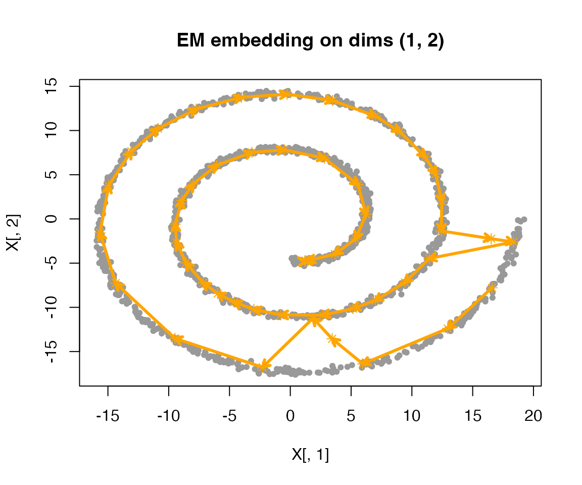

plot(fit_ml, plot_type = "elbo")