Anlysis of Prior Sensitivity for sGP Models
Ziang Zhang
2024-11-21
Last updated: 2024-12-06
Checks: 7 0
Knit directory: online_tut/
This reproducible R Markdown analysis was created with workflowr (version 1.7.1). The Checks tab describes the reproducibility checks that were applied when the results were created. The Past versions tab lists the development history.
Great! Since the R Markdown file has been committed to the Git repository, you know the exact version of the code that produced these results.
Great job! The global environment was empty. Objects defined in the global environment can affect the analysis in your R Markdown file in unknown ways. For reproduciblity it’s best to always run the code in an empty environment.
The command set.seed(20241120) was run prior to running
the code in the R Markdown file. Setting a seed ensures that any results
that rely on randomness, e.g. subsampling or permutations, are
reproducible.
Great job! Recording the operating system, R version, and package versions is critical for reproducibility.
Nice! There were no cached chunks for this analysis, so you can be confident that you successfully produced the results during this run.
Great job! Using relative paths to the files within your workflowr project makes it easier to run your code on other machines.
Great! You are using Git for version control. Tracking code development and connecting the code version to the results is critical for reproducibility.
The results in this page were generated with repository version 45c843e. See the Past versions tab to see a history of the changes made to the R Markdown and HTML files.
Note that you need to be careful to ensure that all relevant files for
the analysis have been committed to Git prior to generating the results
(you can use wflow_publish or
wflow_git_commit). workflowr only checks the R Markdown
file, but you know if there are other scripts or data files that it
depends on. Below is the status of the Git repository when the results
were generated:
Ignored files:
    Ignored:    .DS_Store
    Ignored:    .Rhistory
    Ignored:    .Rproj.user/
    Ignored:    analysis/.DS_Store
    Ignored:    analysis/.Rhistory
    Ignored:    code/.DS_Store

Untracked files:
    Untracked:  analysis/_includes/

Unstaged changes:
    Modified:   analysis/_site.yml
Note that any generated files, e.g. HTML, png, CSS, etc., are not included in this status report because it is ok for generated content to have uncommitted changes.
These are the previous versions of the repository in which changes were
made to the R Markdown (analysis/sensitivity.rmd) and HTML
(docs/sensitivity.html) files. If you’ve configured a
remote Git repository (see ?wflow_git_remote), click on the
hyperlinks in the table below to view the files as they were in that
past version.
| File | Version | Author | Date | Message |
|---|---|---|---|---|
| html | fd909de | Ziang Zhang | 2024-11-26 | Build site. |
| Rmd | c245474 | Ziang Zhang | 2024-11-26 | workflowr::wflow_publish("analysis/sensitivity.rmd") |
| html | 814c6ba | Ziang Zhang | 2024-11-26 | Build site. |
| Rmd | 9cc5214 | Ziang Zhang | 2024-11-26 | workflowr::wflow_publish("analysis/sensitivity.rmd") |
| html | d296bb4 | Ziang Zhang | 2024-11-24 | Build site. |
| Rmd | 77ac328 | Ziang Zhang | 2024-11-24 | workflowr::wflow_publish("analysis/sensitivity.rmd") |
| html | 0218bdf | Ziang Zhang | 2024-11-21 | Build site. |
| Rmd | b6729c1 | Ziang Zhang | 2024-11-21 | workflowr::wflow_publish("analysis/sensitivity.rmd") |
library(tidyverse)── Attaching core tidyverse packages ──────────────────────── tidyverse 2.0.0 ──
✔ dplyr 1.1.4 ✔ readr 2.1.5
✔ forcats 1.0.0 ✔ stringr 1.5.1
✔ ggplot2 3.5.1 ✔ tibble 3.2.1
✔ lubridate 1.9.3 ✔ tidyr 1.3.1
✔ purrr 1.0.2
── Conflicts ────────────────────────────────────────── tidyverse_conflicts() ──
✖ dplyr::filter() masks stats::filter()
✖ dplyr::lag() masks stats::lag()
ℹ Use the conflicted package (<http://conflicted.r-lib.org/>) to force all conflicts to become errorslibrary(BayesGP)Introduction
One important factor that affects the inference of the sGP model is the choice of the prior on its SD parameter \(\sigma\). The suggested way to construct prior on \(\sigma\) is through an Exponential prior on its \(h\)-step predictive SD \(\sigma(h)\), with the form of \[ \text{P}[\sigma(h)>u] = 0.5, \] where \(u\) is prior median.
In this tutorial, we will examine the sensitivity of the sGP model to the choice of the prior on \(\sigma\) by fitting the model to the Lynx dataset with different priors on \(\sigma\).
data <- data.frame(year = seq(1821, 1934, by = 1), logy = log(as.numeric(lynx)), y = as.numeric(lynx))
data$x <- data$year - min(data$year)
x <- data$x
y <- data$y
data_reduced <- data[1:80,]
test_data <- data[-c(1:80),]
### Region of prediction
region_lynx <- c(1821,1960)
Varying the threshold
First, we write a function that takes in the prior median
u and fits the sGP model with the corresponding prior on
\(\sigma(50)\), and then returns the
posterior summary of the fitted model.
fit_once <- function(u, alpha = 0.5){
  pred_SD <- list(u = u, alpha = alpha)
  results_sGP <- BayesGP::model_fit(
    formula = y ~ f(x = year, model = "sgp", k = 30,
                    period = 10,
                    sd.prior = list(param = pred_SD, h = 50),
                    initial_location = "left", region = region_lynx) +
      f(x = x, model = "IID", sd.prior = list(param = list(u = 1, alpha = 0.5))),
    data = data_reduced,
    family = "poisson")
  pred_g1 <- predict(results_sGP, newdata = data.frame(x = x, year = data$year), variable = "year", include.intercept = T, quantiles = c(0.1,0.9))
  return(pred_g1)
}
Let’s try different values of \(u\):
alpha = 0.5
u_vec = c(0.01, 0.03, 0.05, 0.1, 0.2, 0.3, 0.4, 0.5, 0.6, 0.8, 1, 1.5, 2)
pred_summary <- lapply(u_vec, fit_once, alpha = alpha)
pred_means <- do.call(rbind, lapply(pred_summary, function(x) x$mean))
Let’s plot the posterior mean
# Create a color palette from light to dark
color_palette <- colorRampPalette(c("lightblue", "blue"))

# Generate colors for the number of `u_vec`
colors <- color_palette(length(u_vec))

plot(data$year, data$logy, type = "p", col = "black", lwd = 2, xlab = "Year", ylab = "Lynx count", cex = 0.1)
matlines(data$year, t(pred_means), col = colors, lty = 1)
legend("topleft", legend = paste("u =", u_vec), col = colors, lty = 1, cex = 1)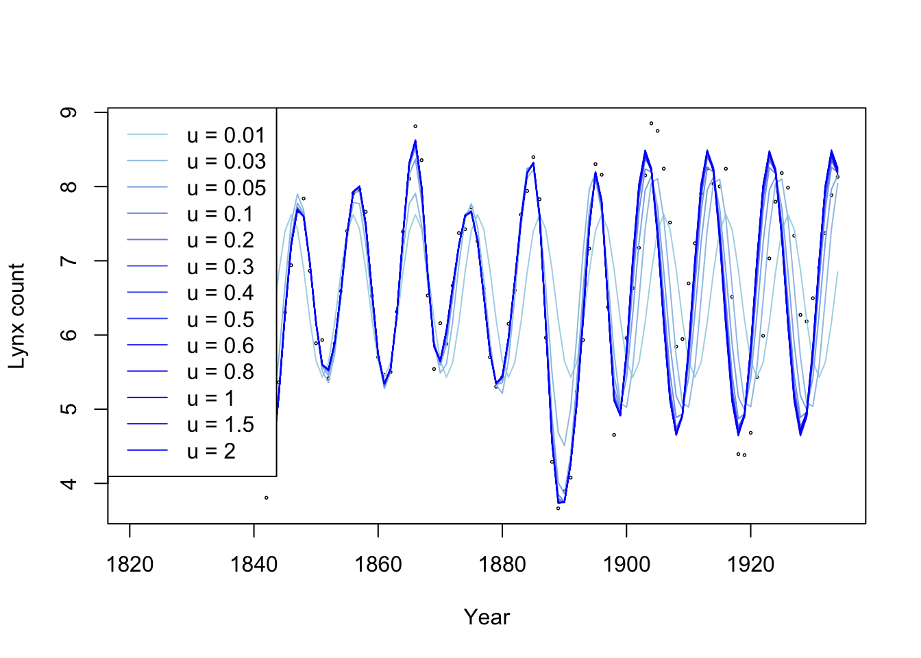
We could also plot the MSE of the posterior mean for different values of \(u\).
MSEs <- apply(pred_means, 1, function(x) mean((x - data$logy)^2))
plot(u_vec, MSEs, type = "o", col = "blue", lwd = 2, xlab = "u", ylab = "MSE")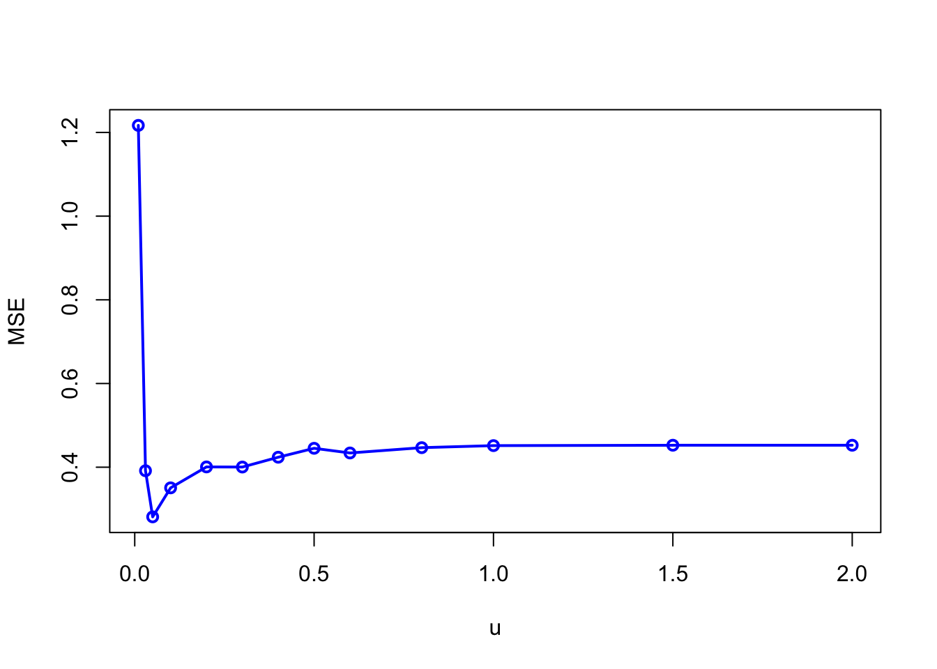
Overall, unless the value of the prior median \(u\) is too small, the MSE is not sensitive to \(u\).
We could similar check how the coverage of the 80% credible interval changes with different values of \(u\).
coverage <- lapply(pred_summary, function(x) mean(data$logy > x$q0.1 & data$logy < x$q0.9))
plot(u_vec, coverage, type = "o", col = "blue", lwd = 2, xlab = "u", ylab = "Coverage", ylim = c(0,1))
abline(h = 0.8, col = "red", lty = "dashed")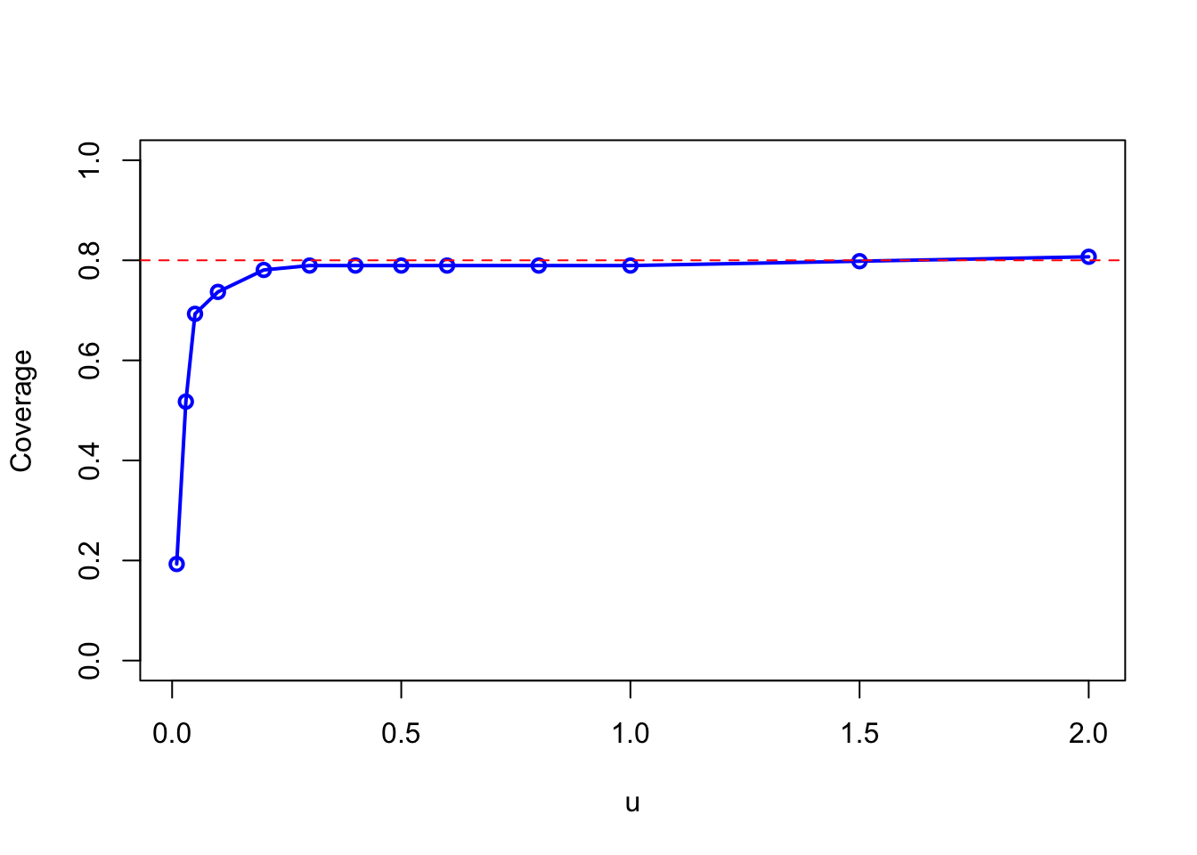
sessionInfo()R version 4.3.1 (2023-06-16)
Platform: aarch64-apple-darwin20 (64-bit)
Running under: macOS Monterey 12.7.4
Matrix products: default
BLAS: /Library/Frameworks/R.framework/Versions/4.3-arm64/Resources/lib/libRblas.0.dylib
LAPACK: /Library/Frameworks/R.framework/Versions/4.3-arm64/Resources/lib/libRlapack.dylib; LAPACK version 3.11.0
locale:
[1] en_US.UTF-8/en_US.UTF-8/en_US.UTF-8/C/en_US.UTF-8/en_US.UTF-8
time zone: America/Chicago
tzcode source: internal
attached base packages:
[1] stats graphics grDevices utils datasets methods base
other attached packages:
[1] BayesGP_0.1.3 lubridate_1.9.3 forcats_1.0.0 stringr_1.5.1
[5] dplyr_1.1.4 purrr_1.0.2 readr_2.1.5 tidyr_1.3.1
[9] tibble_3.2.1 ggplot2_3.5.1 tidyverse_2.0.0 workflowr_1.7.1
loaded via a namespace (and not attached):
[1] gtable_0.3.6 TMB_1.9.15 xfun_0.48
[4] bslib_0.8.0 ks_1.14.3 processx_3.8.4
[7] lattice_0.22-6 numDeriv_2016.8-1.1 callr_3.7.6
[10] tzdb_0.4.0 bitops_1.0-9 vctrs_0.6.5
[13] tools_4.3.1 ps_1.8.0 generics_0.1.3
[16] aghq_0.4.1 fansi_1.0.6 highr_0.11
[19] cluster_2.1.6 pkgconfig_2.0.3 fds_1.8
[22] Matrix_1.6-4 KernSmooth_2.23-24 data.table_1.16.2
[25] lifecycle_1.0.4 compiler_4.3.1 git2r_0.33.0
[28] statmod_1.5.0 munsell_0.5.1 getPass_0.2-4
[31] mvQuad_1.0-8 httpuv_1.6.15 htmltools_0.5.8.1
[34] rainbow_3.8 sass_0.4.9 RCurl_1.98-1.16
[37] yaml_2.3.10 pracma_2.4.4 later_1.3.2
[40] pillar_1.9.0 jquerylib_0.1.4 whisker_0.4.1
[43] MASS_7.3-60 cachem_1.1.0 mclust_6.1.1
[46] tidyselect_1.2.1 digest_0.6.37 mvtnorm_1.3-1
[49] stringi_1.8.4 splines_4.3.1 pcaPP_2.0-5
[52] rprojroot_2.0.4 fastmap_1.2.0 grid_4.3.1
[55] colorspace_2.1-1 cli_3.6.3 magrittr_2.0.3
[58] utf8_1.2.4 withr_3.0.2 scales_1.3.0
[61] promises_1.3.0 timechange_0.3.0 rmarkdown_2.28
[64] httr_1.4.7 deSolve_1.40 hms_1.1.3
[67] evaluate_1.0.1 knitr_1.48 rlang_1.1.4
[70] Rcpp_1.0.13-1 hdrcde_3.4 glue_1.8.0
[73] fda_6.2.0 rstudioapi_0.16.0 jsonlite_1.8.9
[76] R6_2.5.1 fs_1.6.4