Plot Method for fash Objects

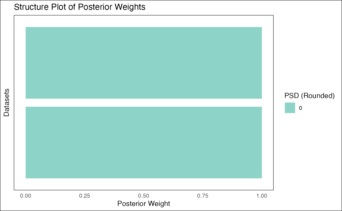
Generates a structure plot of the posterior weights stored in the fash object, visualizing the distribution of posterior weights across datasets and PSD values.

# S3 method for class 'fash'
plot(x, ordering = NULL, discrete = FALSE, ...)

Arguments

x

A fash object containing the results of the FASH pipeline.

ordering

A character string specifying the method for reordering datasets (e.g., "mean" or "lfdr").

- "mean": Reorder by the mean of the posterior PSD.

- "lfdr": Reorder by the local false discovery rate.

- NULL: No reordering (default).

discrete

A logical value. If TRUE, treats PSD values as discrete categories with distinct colors. If FALSE, treats PSD values as a continuous variable with a gradient.

...

Additional arguments passed to fash_structure_plot.

Examples

set.seed(1)
data_list <- list(
  data.frame(y = rpois(5, lambda = 5), x = 1:5, offset = 0),
  data.frame(y = rpois(5, lambda = 5), x = 1:5, offset = 0)
)
S <- NULL
Omega <- NULL
grid <- seq(0, 2, length.out = 10)
fash_obj <- fash(data_list = data_list, Y = "y", smooth_var = "x", offset = "offset", S = S, Omega = Omega, grid = grid, likelihood = "poisson", verbose = TRUE)
#> Starting data setup...
#> Completed data setup in 0.00 seconds.
#> Starting likelihood computation...
#> 
  |                                                                            
  |                                                                      |   0%
  |                                                                            
  |===================================                                   |  50%
  |                                                                            
  |======================================================================| 100%
#> Completed likelihood computation in 0.15 seconds.
#> Starting empirical Bayes estimation...
#> Completed empirical Bayes estimation in 0.00 seconds.
#> fash object created successfully.
plot(fash_obj, ordering = "mean", discrete = TRUE)