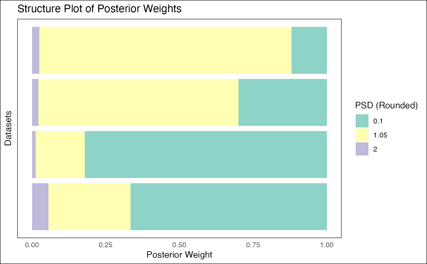
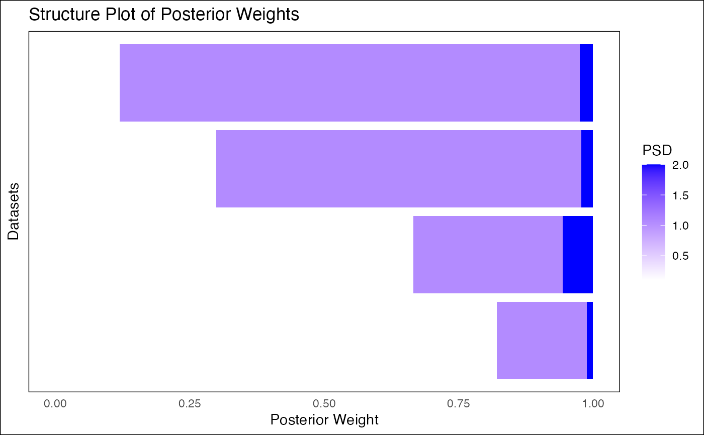
Structure Plot for Posterior Weights — fash_structure

This function takes the output of fash_eb_est and generates a structure plot visualizing the posterior weights for all datasets. It can display PSD values as either continuous or discrete variables and optionally reorder datasets.

fash_structure_plot(
  eb_output,
  discrete = FALSE,
  ordering = NULL,
  selected_indices = NULL
)

Arguments

eb_output

A list output from fash_eb_est, containing:

posterior_weight: A numeric matrix of posterior weights (datasets as rows, PSD as columns).
prior_weight: A data frame of prior weights (not used in this plot).

discrete

A logical value. If TRUE, treats PSD values as discrete categories with distinct colors. If FALSE, treats PSD values as a continuous variable with a gradient.

ordering

A character string specifying the method for reordering datasets. Options are:

NULL: No reordering (default).
`mean`: Reorder by the mean of the posterior PSD.
`median`: Reorder by the median of the posterior PSD.
`lfdr`: Reorder by the local false discovery rate (posterior probability of PSD = 0).

selected_indices

A numeric vector specifying the indices of datasets to display. If NULL, displays all datasets.

Value

A ggplot object representing the structure plot.

Examples

# Example usage
set.seed(1)
grid <- seq(0.1, 2, length.out = 5)
L_matrix <- matrix(rnorm(20), nrow = 4, ncol = 5)
eb_output <- fash_eb_est(L_matrix, penalty = 2, grid = grid)
plot_cont <- fash_structure_plot(eb_output, discrete = FALSE, ordering = "mean")
plot_disc <- fash_structure_plot(eb_output, discrete = TRUE, ordering = "median")
print(plot_cont)

print(plot_disc)