Infering latent ordering from the pancrea dataset

workflowr

• Summary
• Checks
• Past versions

Last updated: 2025-07-10

Checks: 7 0

Knit directory: InferOrder/

This reproducible R Markdown analysis was created with workflowr (version 1.7.1). The Checks tab describes the reproducibility checks that were applied when the results were created. The Past versions tab lists the development history.

---

R Markdown file: up-to-date

Great! Since the R Markdown file has been committed to the Git repository, you know the exact version of the code that produced these results.

Environment: empty

Great job! The global environment was empty. Objects defined in the global environment can affect the analysis in your R Markdown file in unknown ways. For reproduciblity it’s best to always run the code in an empty environment.

Seed: set.seed(20250707)

The command set.seed(20250707) was run prior to running the code in the R Markdown file. Setting a seed ensures that any results that rely on randomness, e.g. subsampling or permutations, are reproducible.

Session information: recorded

Great job! Recording the operating system, R version, and package versions is critical for reproducibility.

Cache: none

Nice! There were no cached chunks for this analysis, so you can be confident that you successfully produced the results during this run.

File paths: relative

Great job! Using relative paths to the files within your workflowr project makes it easier to run your code on other machines.

Repository version: 032918c

Great! You are using Git for version control. Tracking code development and connecting the code version to the results is critical for reproducibility.

The results in this page were generated with repository version 032918c. See the Past versions tab to see a history of the changes made to the R Markdown and HTML files.

Note that you need to be careful to ensure that all relevant files for the analysis have been committed to Git prior to generating the results (you can use wflow_publish or wflow_git_commit). workflowr only checks the R Markdown file, but you know if there are other scripts or data files that it depends on. Below is the status of the Git repository when the results were generated:

Ignored files:
    Ignored:    .DS_Store
    Ignored:    .Rhistory
    Ignored:    .Rproj.user/
    Ignored:    analysis/.DS_Store

Unstaged changes:
    Modified:   code/general_EM.R
    Modified:   code/general_EM_obs.R
    Modified:   code/linear_EM.R

Note that any generated files, e.g. HTML, png, CSS, etc., are not included in this status report because it is ok for generated content to have uncommitted changes.

---

These are the previous versions of the repository in which changes were made to the R Markdown (analysis/explore_pancrea.rmd) and HTML (docs/explore_pancrea.html) files. If you’ve configured a remote Git repository (see ?wflow_git_remote), click on the hyperlinks in the table below to view the files as they were in that past version.

File	Version	Author	Date	Message
Rmd	032918c	Ziang Zhang	2025-07-10	workflowr::wflow_publish("analysis/explore_pancrea.rmd")
html	29aee93	Ziang Zhang	2025-07-09	Build site.
Rmd	e4aadb0	Ziang Zhang	2025-07-09	workflowr::wflow_publish("analysis/explore_pancrea.rmd")
html	dbcdf9a	Ziang Zhang	2025-07-08	Build site.
Rmd	9867260	Ziang Zhang	2025-07-08	workflowr::wflow_publish("analysis/explore_pancrea.rmd")
html	2f5e139	Ziang Zhang	2025-07-08	Build site.
Rmd	27f1ee5	Ziang Zhang	2025-07-08	workflowr::wflow_publish("analysis/explore_pancrea.rmd")

---

Ordering structure plot

Given a set of loadings, we want to infer a latent ordering, that will produce a smooth structure plot.

Data

In this study, we will consider the pancrea dataset studied in here.

For simplicity, we will use the loadings from the semi-NMF, considering only the factors that are most relevant to the cell types, and only a subset of cells with a specific batch type (inDrop3).

library(tibble)
library(tidyr)
library(ggplot2)

Warning: package 'ggplot2' was built under R version 4.3.3

library(Rtsne)
library(umap)
set.seed(1)
source("./code/plot_ordering.R")
load("./data/loading_order/pancreas_factors.rdata")
load("./data/loading_order/pancreas.rdata")
cells <- subsample_cell_types(sample_info$celltype,n = 500)
Loadings <- fl_snmf_ldf$L[cells,c(3,8,9,12,17,18,20,21)]
celltype <- as.character(sample_info$celltype[cells])
names(celltype) <- rownames(Loadings)
batchtype <- as.character(sample_info$tech[cells])
names(batchtype) <- rownames(Loadings)

# Let's further restrict cells to only contain cells from one type of batch
Loadings <- Loadings[batchtype == "inDrop3",]
celltype <- celltype[batchtype == "inDrop3"]
batchtype <- batchtype[batchtype == "inDrop3"]

Let’s start with an un-ordered structure plot.

plot_structure(Loadings)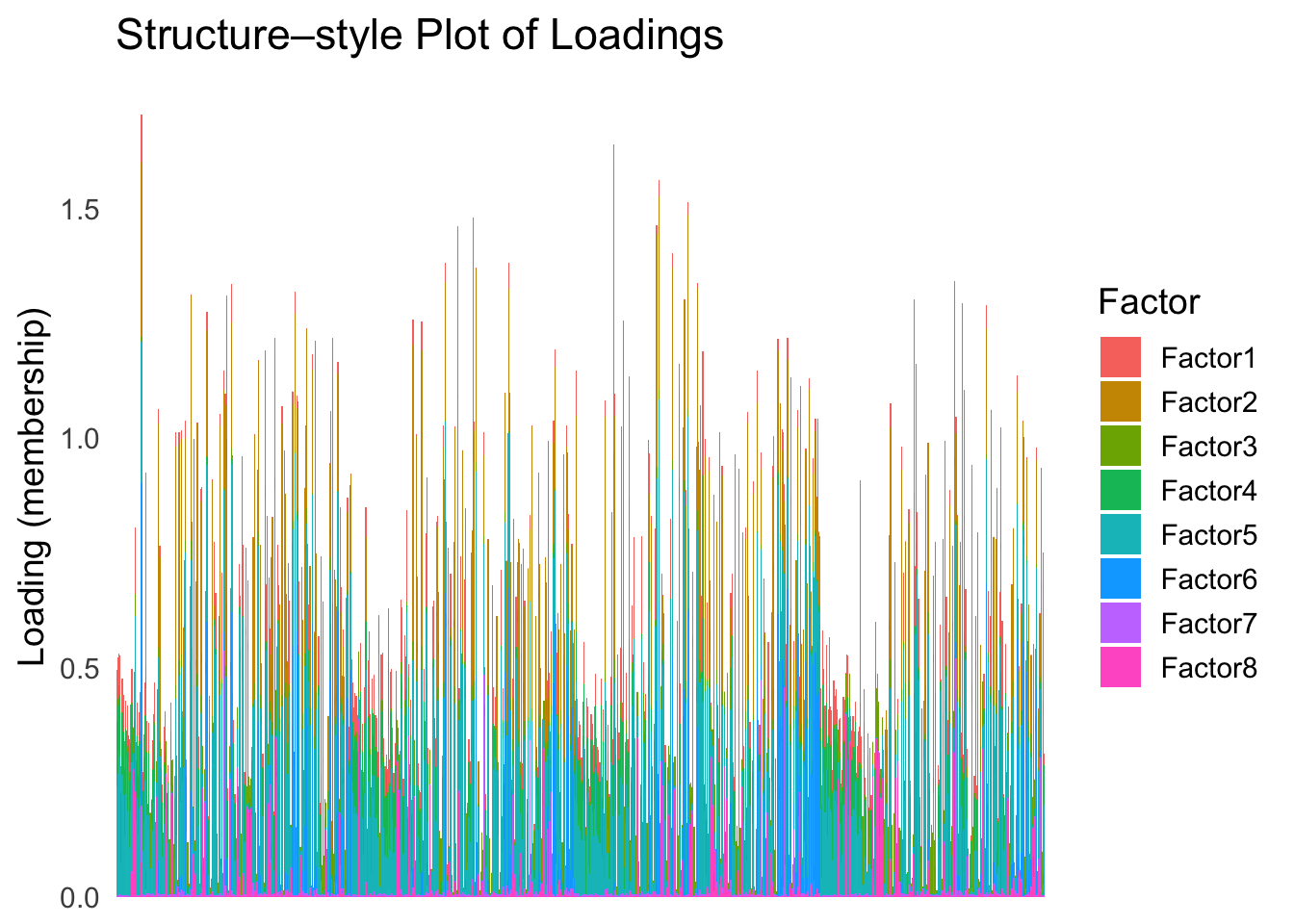

Past versions of unnamed-chunk-3-1.png

Version	Author	Date
2f5e139	Ziang Zhang	2025-07-08

First PC

Now, let’s see how does the result look like when we order the structure plot by the first PC.

PC1 <- prcomp(Loadings,center = TRUE, scale. = FALSE)$x[,1]
PC1_order <- order(PC1)
plot_structure(Loadings, order = rownames(Loadings)[PC1_order])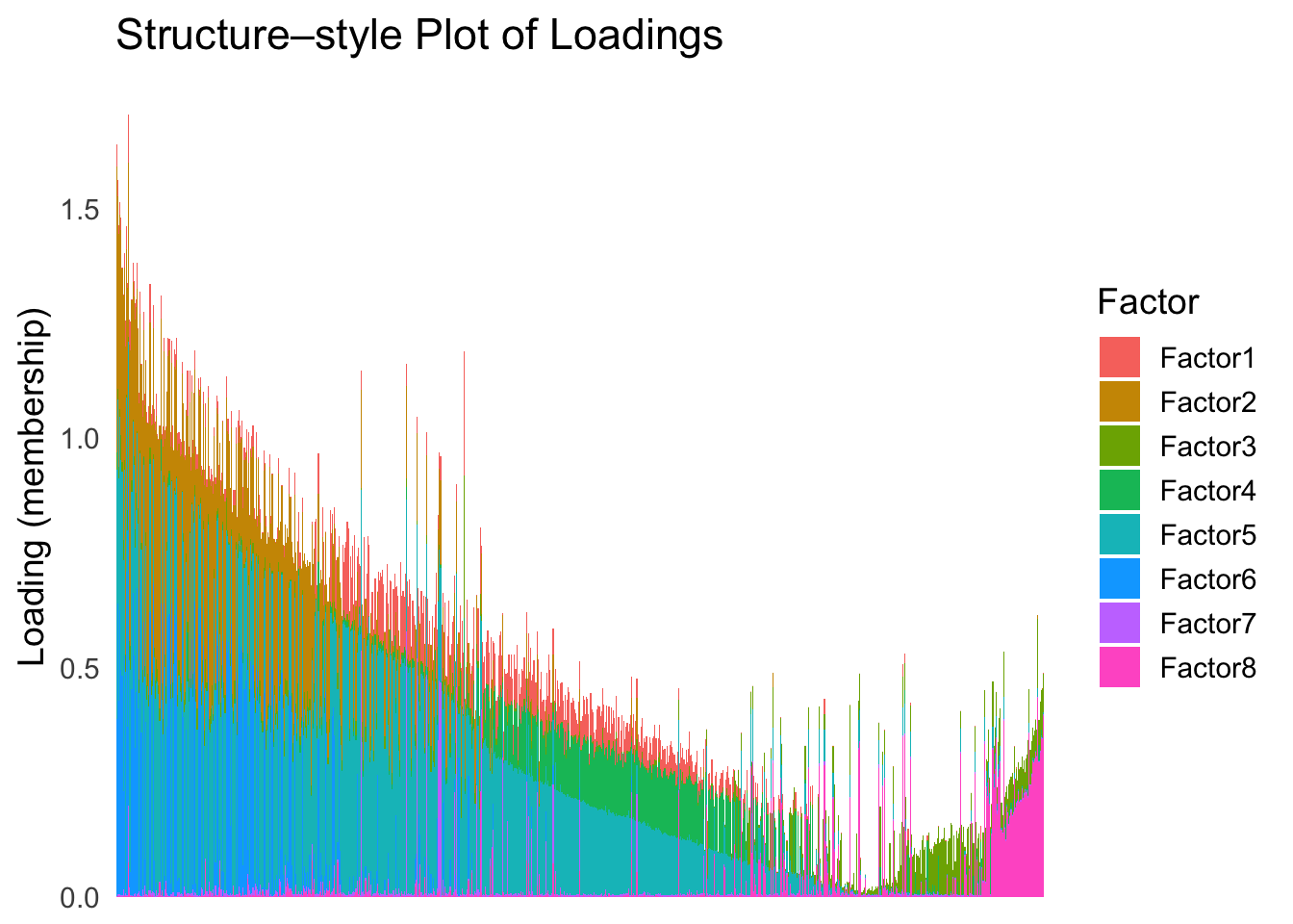

Past versions of unnamed-chunk-4-1.png

Version	Author	Date
2f5e139	Ziang Zhang	2025-07-08

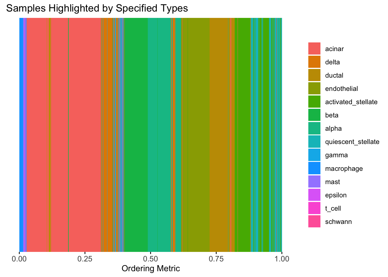
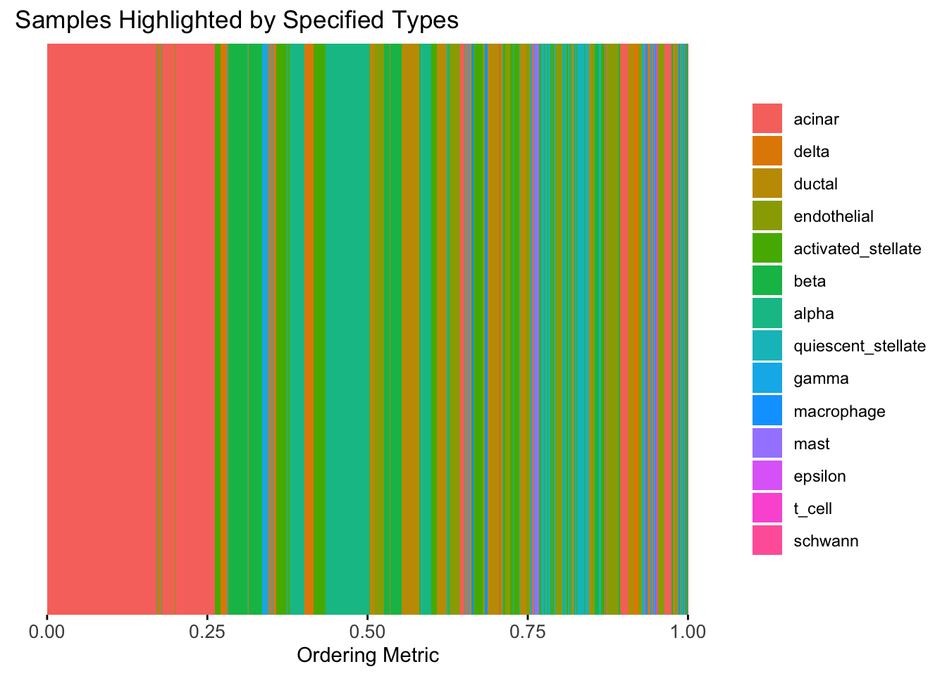
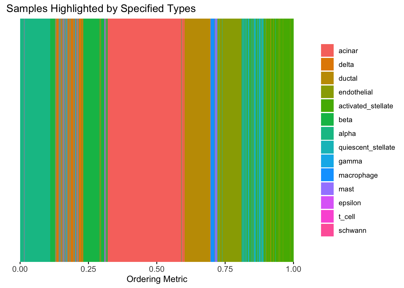
Take a look at the ordering metric versus the cell types.

# highlights <- c("acinar","ductal","delta","gamma", "macrophage", "endothelial")
highlights <- unique(celltype)
PC1 <- prcomp(Loadings,center = TRUE, scale. = FALSE)$x[,1]
plot_highlight_types(type_vec = celltype,
                     subset_types = highlights,
                     ordering_metric = PC1,
                     other_color = "white"
                     )

Warning: `position_stack()` requires non-overlapping x intervals.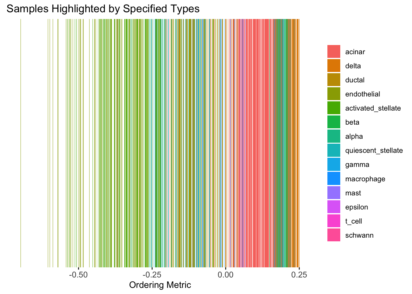

Past versions of unnamed-chunk-5-1.png

Version	Author	Date
2f5e139	Ziang Zhang	2025-07-08

Here the x-axis represents the latent ordering of each cell, and the color represents its cell type. Based on this figure, it appears the first PC distinguishes between (delta, gamma) and (acinar, ductal). However, the ordering could not tell the difference between delta and gamma. Also, the ordering could not distinguish the macrophage from other cell types.

We could also take a look at the distribution of the latent ordering metric for each cell type.

distribution_highlight_types(
  type_vec        = celltype,
  subset_types    = highlights,
  ordering_metric = PC1,
  density         = FALSE
)

Warning: Groups with fewer than two datapoints have been dropped.
ℹ Set `drop = FALSE` to consider such groups for position adjustment purposes.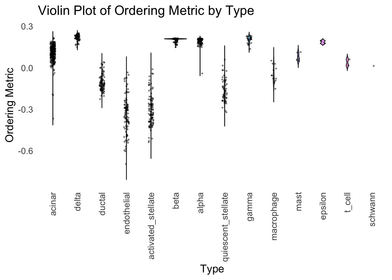

Past versions of unnamed-chunk-6-1.png

Version	Author	Date
2f5e139	Ziang Zhang	2025-07-08

The ordering just based on the first PC seems to be not bad. Further since the PC has a probabilistic interpretation, the ordering can also be interpreted probabilistically.

tSNE

Just as a comparison, let’s see how does the result look like when we order the structure plot by the first tSNE.

set.seed(1)
tsne <- Rtsne(Loadings, dims = 1, perplexity = 30, verbose = TRUE, check_duplicates = FALSE)

Performing PCA
Read the 865 x 8 data matrix successfully!
Using no_dims = 1, perplexity = 30.000000, and theta = 0.500000
Computing input similarities...
Building tree...
Done in 0.03 seconds (sparsity = 0.125422)!
Learning embedding...
Iteration 50: error is 61.378493 (50 iterations in 0.03 seconds)
Iteration 100: error is 53.621893 (50 iterations in 0.03 seconds)
Iteration 150: error is 51.570417 (50 iterations in 0.03 seconds)
Iteration 200: error is 50.534836 (50 iterations in 0.03 seconds)
Iteration 250: error is 49.880683 (50 iterations in 0.03 seconds)
Iteration 300: error is 0.892290 (50 iterations in 0.03 seconds)
Iteration 350: error is 0.620483 (50 iterations in 0.03 seconds)
Iteration 400: error is 0.536455 (50 iterations in 0.03 seconds)
Iteration 450: error is 0.508706 (50 iterations in 0.03 seconds)
Iteration 500: error is 0.487135 (50 iterations in 0.03 seconds)
Iteration 550: error is 0.475625 (50 iterations in 0.03 seconds)
Iteration 600: error is 0.463845 (50 iterations in 0.03 seconds)
Iteration 650: error is 0.453710 (50 iterations in 0.03 seconds)
Iteration 700: error is 0.446554 (50 iterations in 0.03 seconds)
Iteration 750: error is 0.439321 (50 iterations in 0.03 seconds)
Iteration 800: error is 0.434766 (50 iterations in 0.03 seconds)
Iteration 850: error is 0.428145 (50 iterations in 0.03 seconds)
Iteration 900: error is 0.424017 (50 iterations in 0.03 seconds)
Iteration 950: error is 0.420721 (50 iterations in 0.03 seconds)
Iteration 1000: error is 0.417580 (50 iterations in 0.03 seconds)
Fitting performed in 0.63 seconds.

tsne_metric <- tsne$Y[,1]
tsne_order <- order(tsne_metric)
names(tsne_metric) <- rownames(Loadings)

plot_structure(Loadings, order = rownames(Loadings)[tsne_order])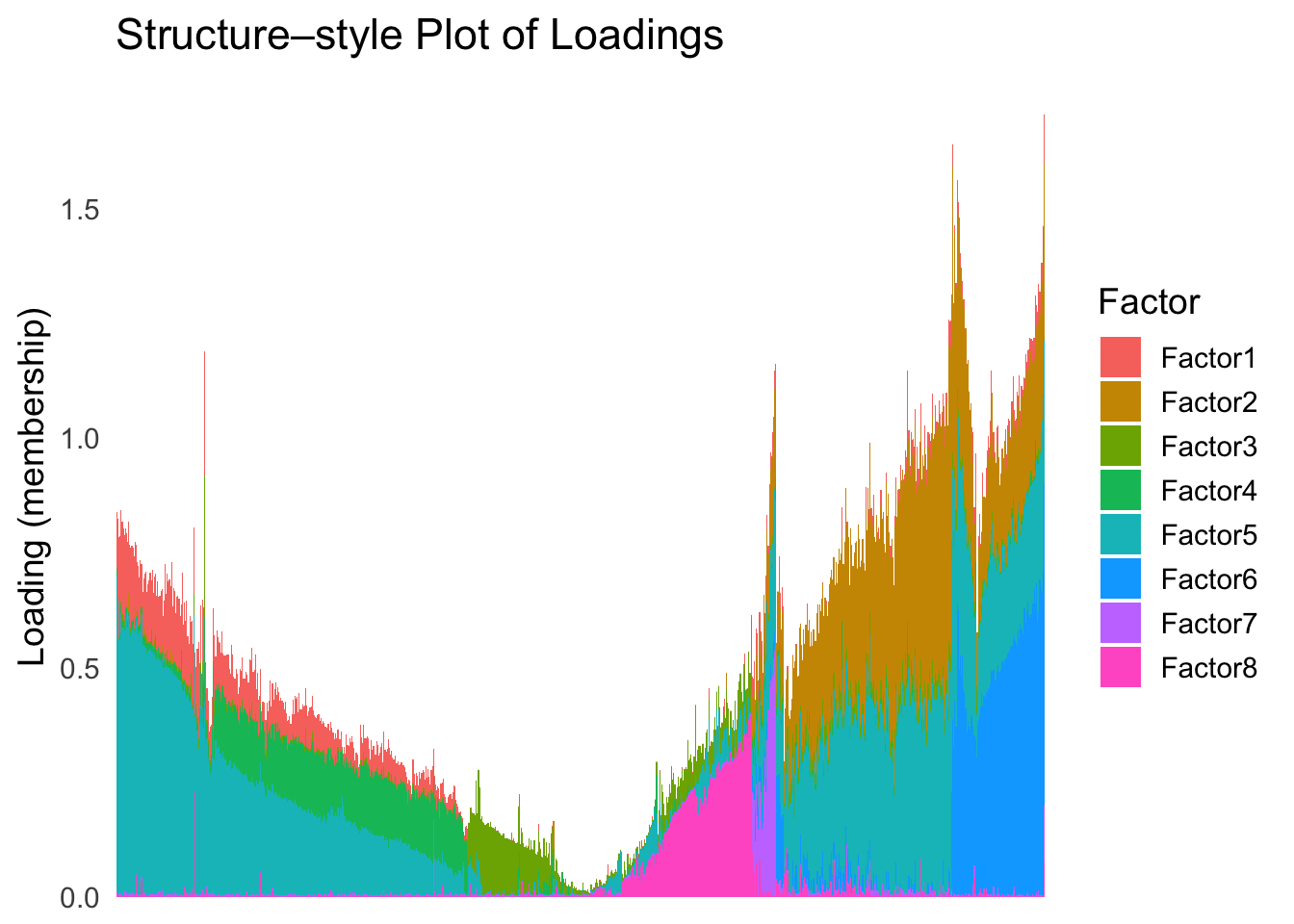

Past versions of unnamed-chunk-8-1.png

Version	Author	Date
2f5e139	Ziang Zhang	2025-07-08

Just based on the structure plot, it seems like the ordering is producing more structured results than the first PC.

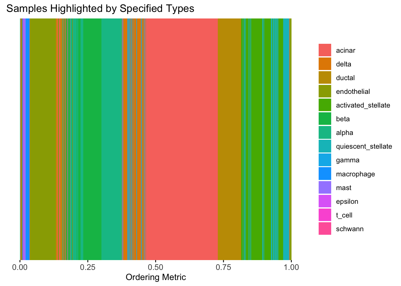
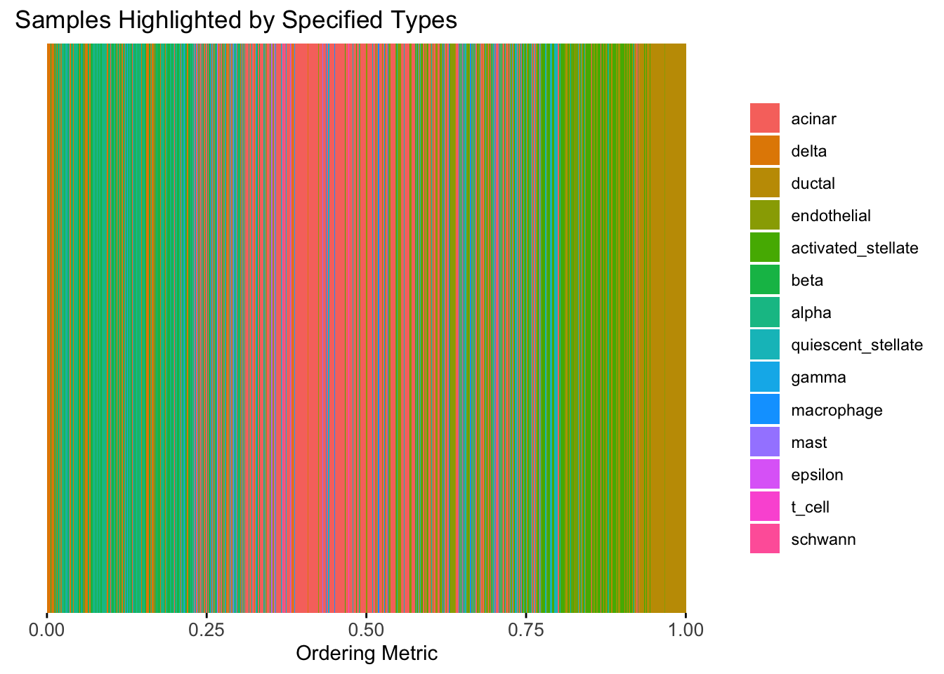
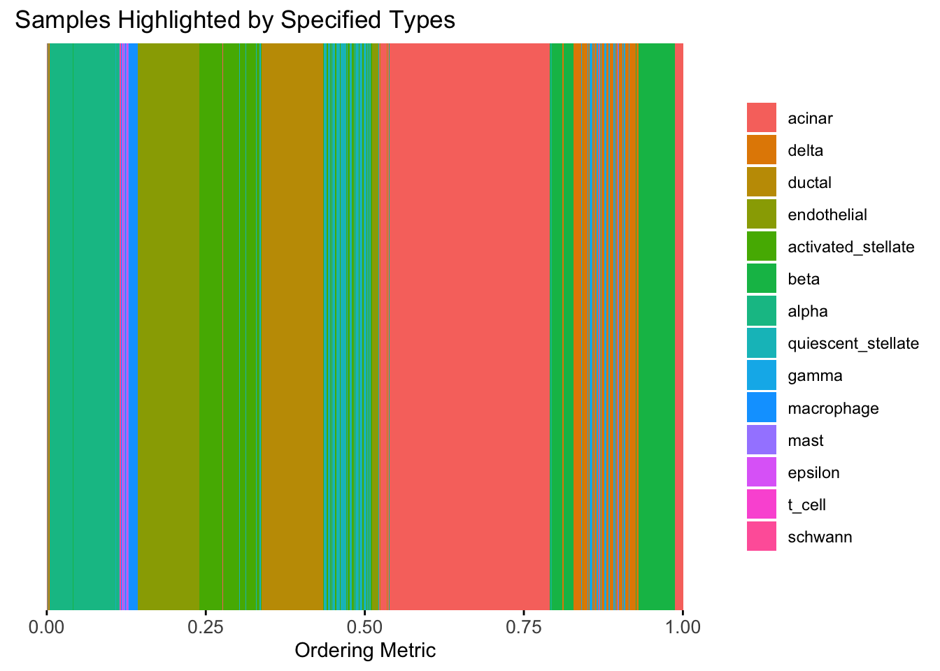
plot_highlight_types(type_vec = celltype,
                     subset_types = highlights,
                     ordering_metric = tsne_metric,
                     other_color = "white"
                     )

Warning: `position_stack()` requires non-overlapping x intervals.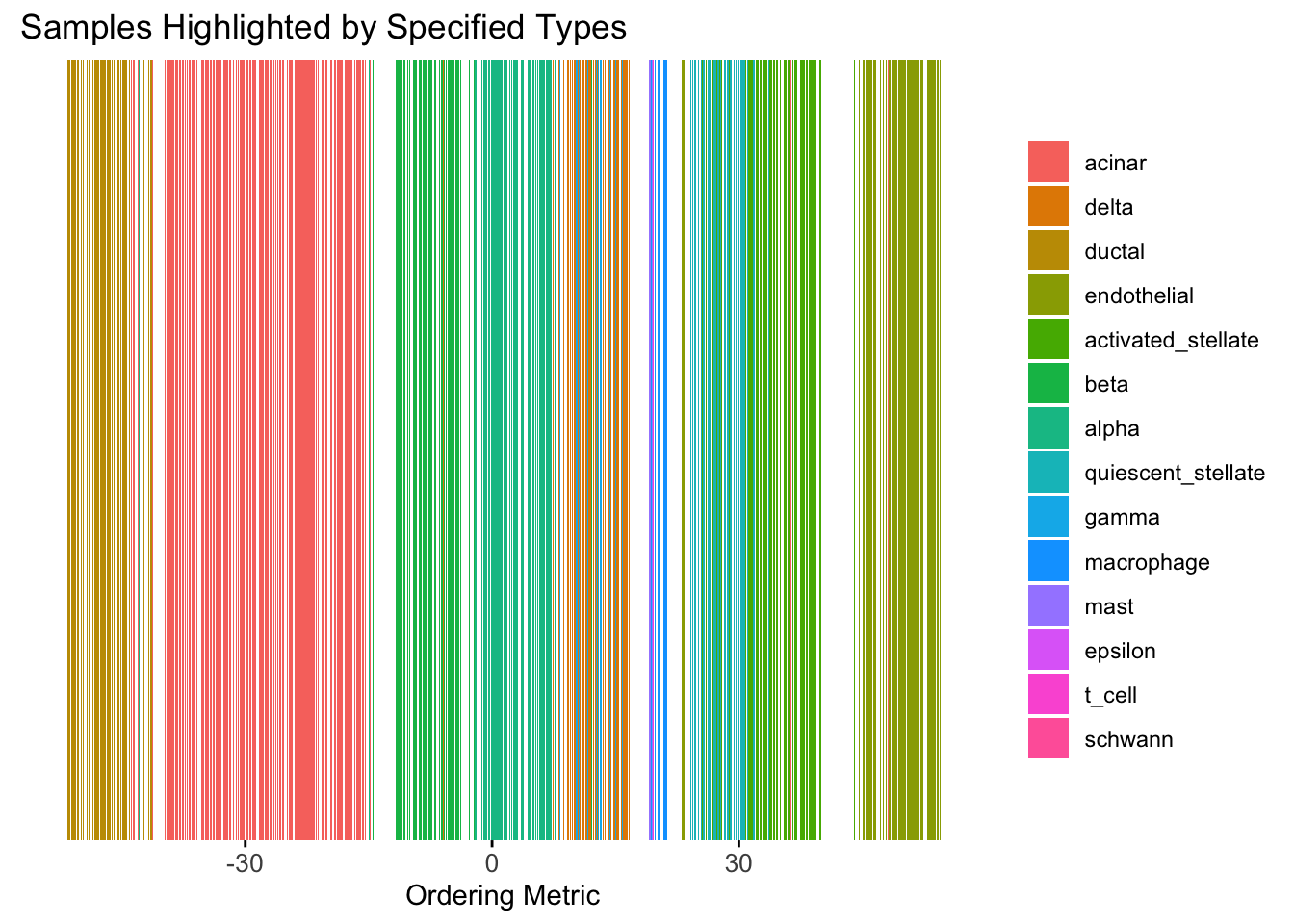

Past versions of unnamed-chunk-9-1.png

Version	Author	Date
2f5e139	Ziang Zhang	2025-07-08

distribution_highlight_types(
  type_vec        = celltype,
  subset_types    = highlights,
  ordering_metric = tsne_metric,
  density         = FALSE
)

Warning: Groups with fewer than two datapoints have been dropped.
ℹ Set `drop = FALSE` to consider such groups for position adjustment purposes.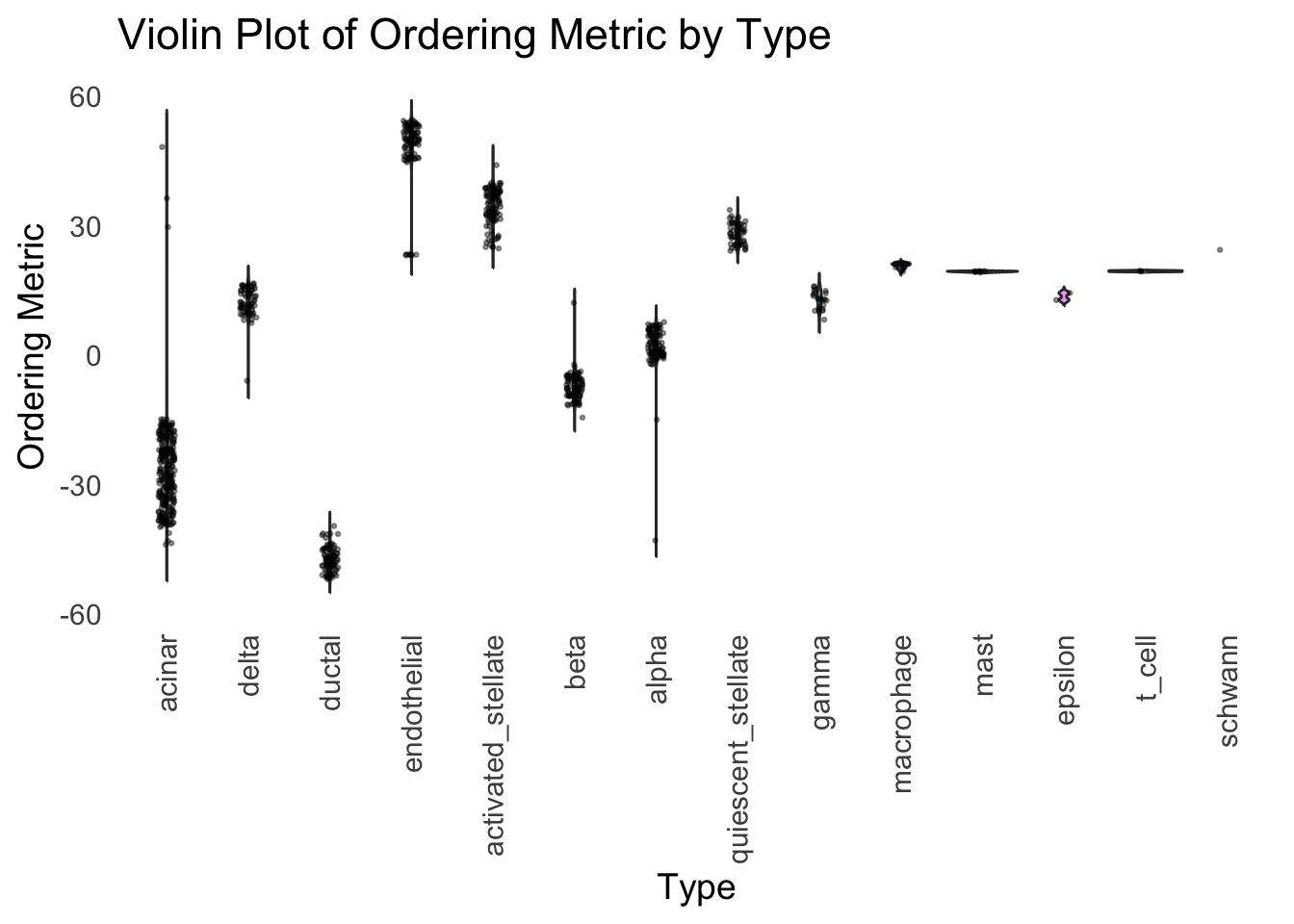

Past versions of unnamed-chunk-10-1.png

Version	Author	Date
2f5e139	Ziang Zhang	2025-07-08

Although the tSNE ordering does not have a clear probabilistic interpretation, the structure produced by this ordering matches the cell types much better than the first PC ordering. The distribution of the ordering metric also shows a clear compact separation between the cell types, which is not the case for the first PC. In particular, the macrophage and endothelial cells are now clearly separated from the other cell types.

However, tSNE’s metric only preserves the local structure of the data, and there is no guarantee that the global distance between the points is preserved in the tSNE metric (e.g. the distance between two groups).

UMAP

Let’s see how does the result look like when we order the structure plot by the first UMAP.

umap_result <- umap(Loadings, n_neighbors = 15, min_dist = 0.1, metric = "euclidean")
umap_metric <- umap_result$layout[,1]
names(umap_metric) <- rownames(Loadings)
umap_order <- order(umap_metric)

plot_structure(Loadings, order = rownames(Loadings)[umap_order])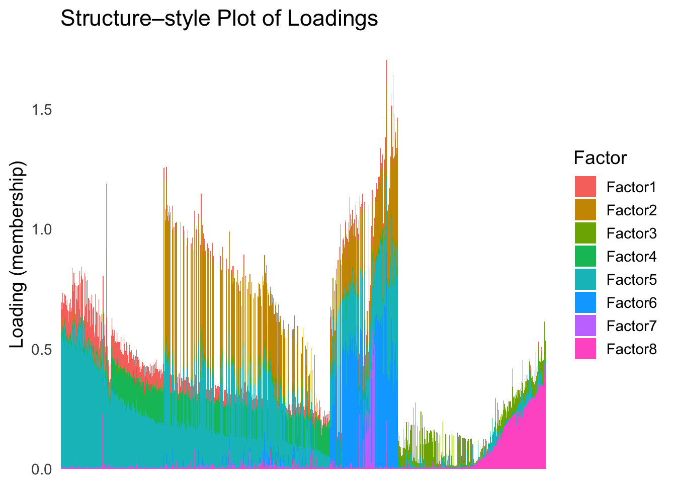

Past versions of unnamed-chunk-12-1.png

Version	Author	Date
2f5e139	Ziang Zhang	2025-07-08

plot_highlight_types(type_vec = celltype,
                     subset_types = highlights,
                     ordering_metric = umap_metric,
                     other_color = "white"
                     )

Warning: `position_stack()` requires non-overlapping x intervals.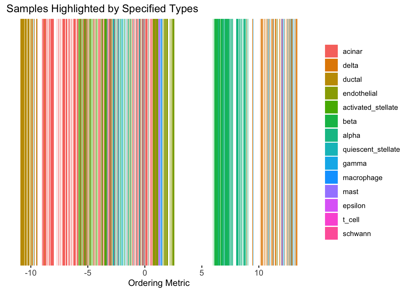

Past versions of unnamed-chunk-13-1.png

Version	Author	Date
2f5e139	Ziang Zhang	2025-07-08

distribution_highlight_types(
  type_vec        = celltype,
  subset_types    = highlights,
  ordering_metric = umap_metric,
  density         = FALSE
)

Warning: Groups with fewer than two datapoints have been dropped.
ℹ Set `drop = FALSE` to consider such groups for position adjustment purposes.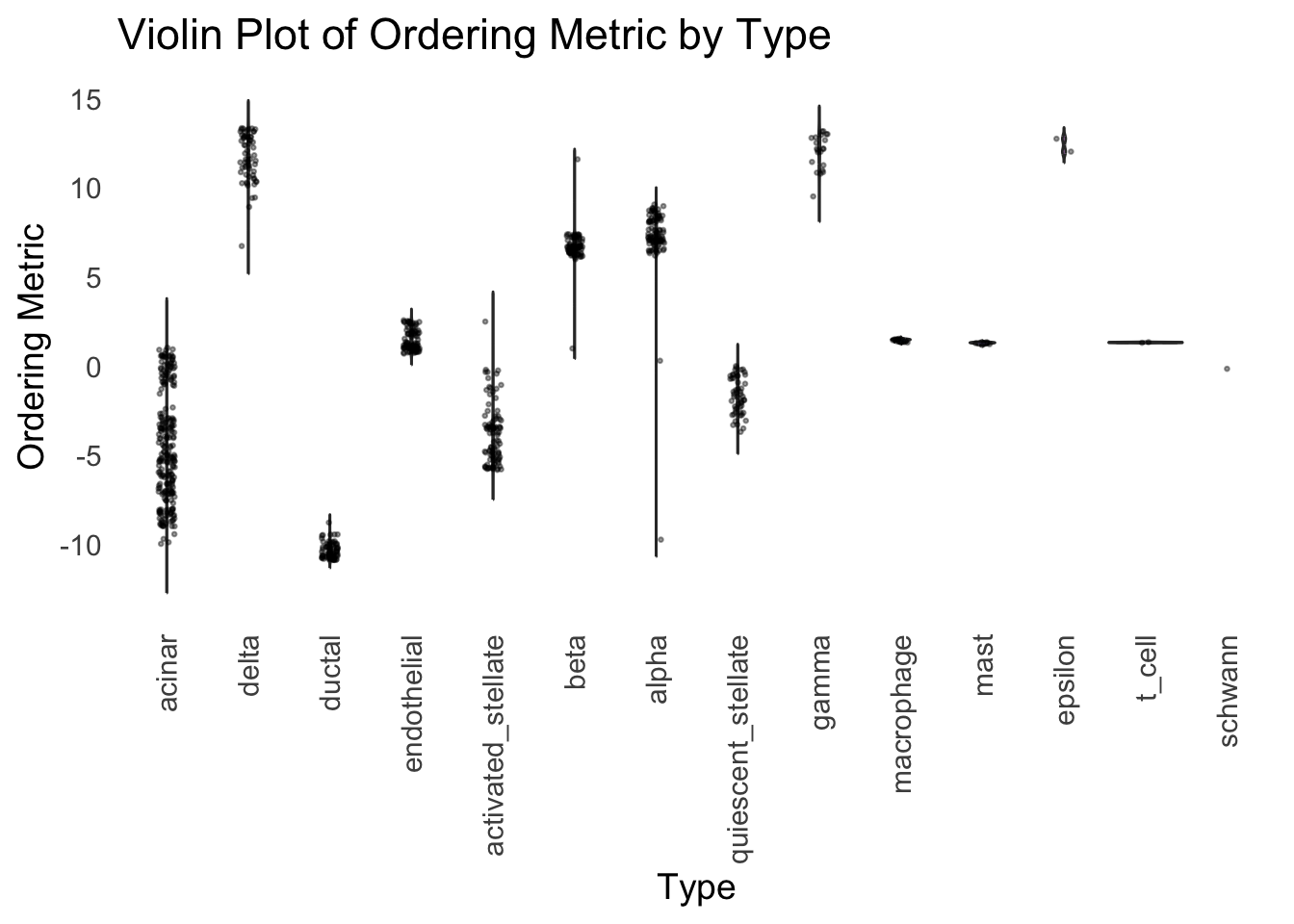

Past versions of unnamed-chunk-14-1.png

Version	Author	Date
2f5e139	Ziang Zhang	2025-07-08

UMAP can also provide very clear separation between the cell types. However, just like tSNE, it does not have a clear probabilistic interpretation. Furthermore, the global ordering structure from UMAP seems to conflict with the global ordering structure from the tSNE. In the tSNE ordering, acinar is next to delta, which is next to endothelial, where as in the UMAP ordering, acinar is next to endothelial, which is next to delta.

The separation of macrophage is not as clear as in the tSNE ordering.

Hierarchical Clustering

Next, let’s try doing hierarchical clustering on the loadings and see how does the result look like when we order the structure plot by the hierarchical clustering.

First, let’s try when method = single.

hc <- hclust(dist(Loadings), method = "single")
hc_order <- hc$order
names(hc_order) <- rownames(Loadings)

plot_structure(Loadings, order = rownames(Loadings)[hc_order])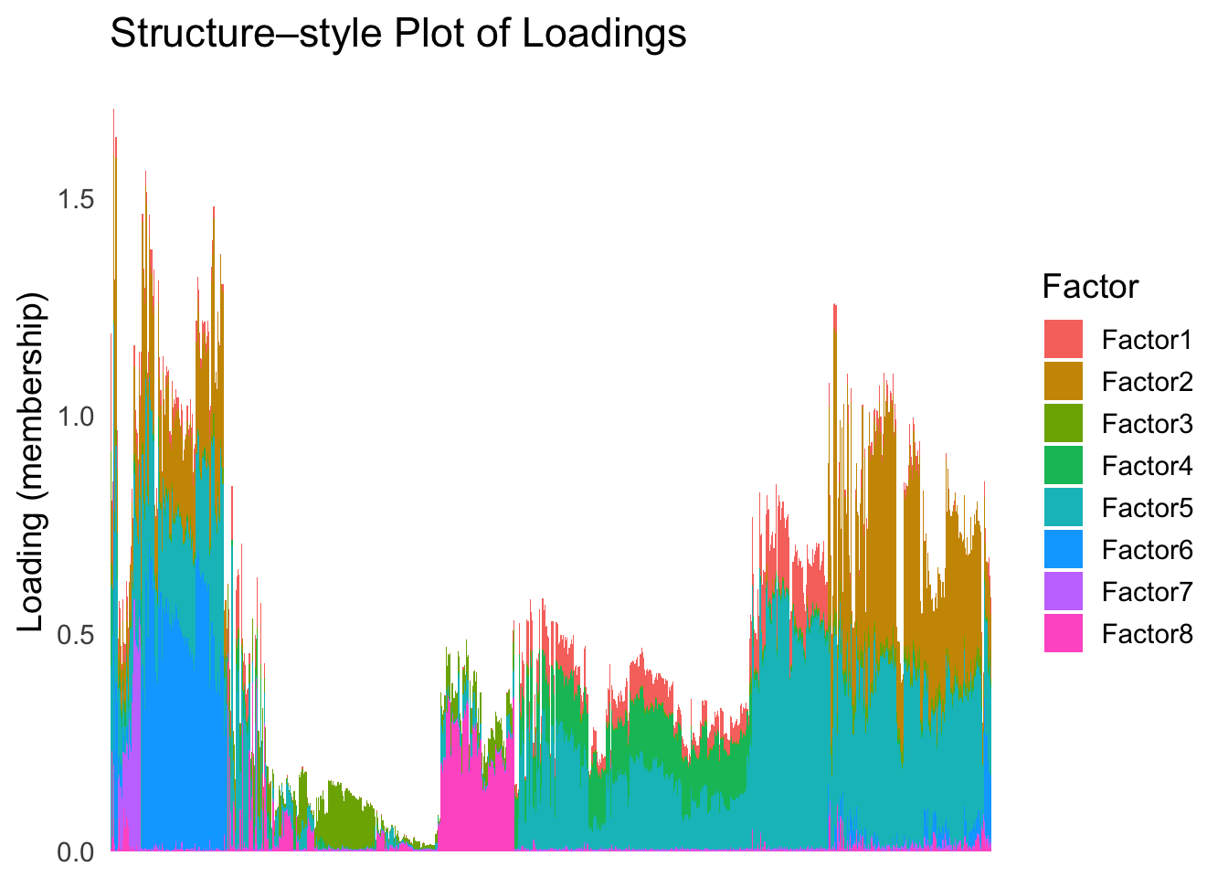

Past versions of unnamed-chunk-16-1.png

Version	Author	Date
2f5e139	Ziang Zhang	2025-07-08

plot_highlight_types(type_vec = celltype,
                     subset_types = highlights,
                     order_vec = rownames(Loadings)[hc_order],
                     other_color = "white"
                     )

Past versions of unnamed-chunk-17-1.png

Version	Author	Date
2f5e139	Ziang Zhang	2025-07-08

distribution_highlight_types(
  type_vec        = celltype,
  subset_types    = highlights,
  order_vec = rownames(Loadings)[hc_order],
  density         = FALSE
)

Warning: Groups with fewer than two datapoints have been dropped.
ℹ Set `drop = FALSE` to consider such groups for position adjustment purposes.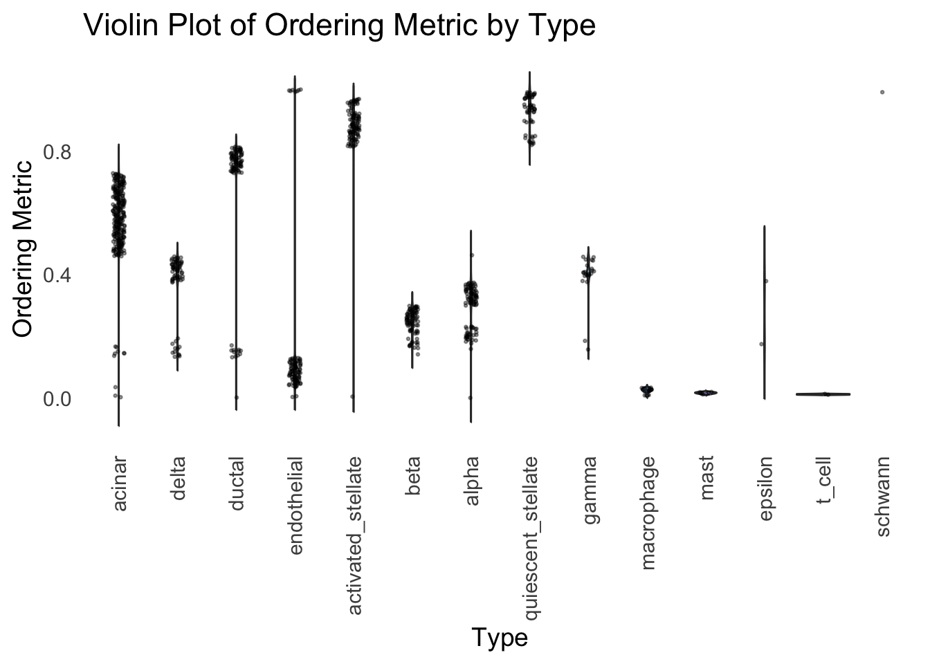

Past versions of unnamed-chunk-18-1.png

Version	Author	Date
2f5e139	Ziang Zhang	2025-07-08

Similar to t-SNE, the hierarchical clustering ordering also produces a clear separation between the cell types.

Then, let’s try when method = ward.D2.

hc <- hclust(dist(Loadings), method = "ward.D2")
hc_order <- hc$order
names(hc_order) <- rownames(Loadings)

plot_structure(Loadings, order = rownames(Loadings)[hc_order])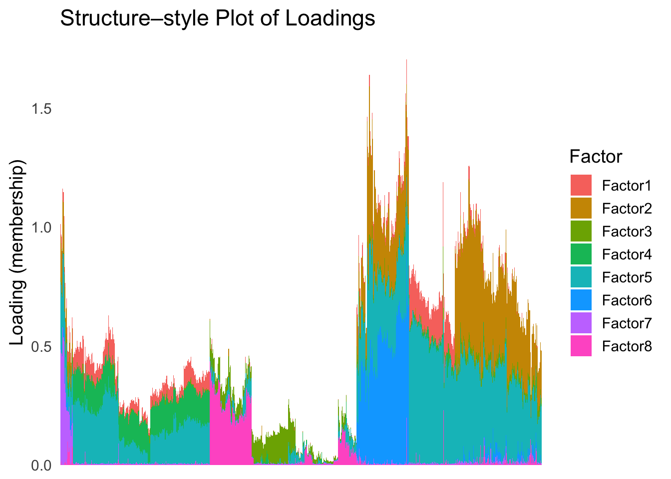

Past versions of unnamed-chunk-20-1.png

Version	Author	Date
2f5e139	Ziang Zhang	2025-07-08

plot_highlight_types(type_vec = celltype,
                     subset_types = highlights,
                     order_vec = rownames(Loadings)[hc_order],
                     other_color = "white"
                     )

Past versions of unnamed-chunk-21-1.png

Version	Author	Date
2f5e139	Ziang Zhang	2025-07-08

distribution_highlight_types(
  type_vec        = celltype,
  subset_types    = highlights,
  order_vec = rownames(Loadings)[hc_order],
  density         = FALSE
)

Warning: Groups with fewer than two datapoints have been dropped.
ℹ Set `drop = FALSE` to consider such groups for position adjustment purposes.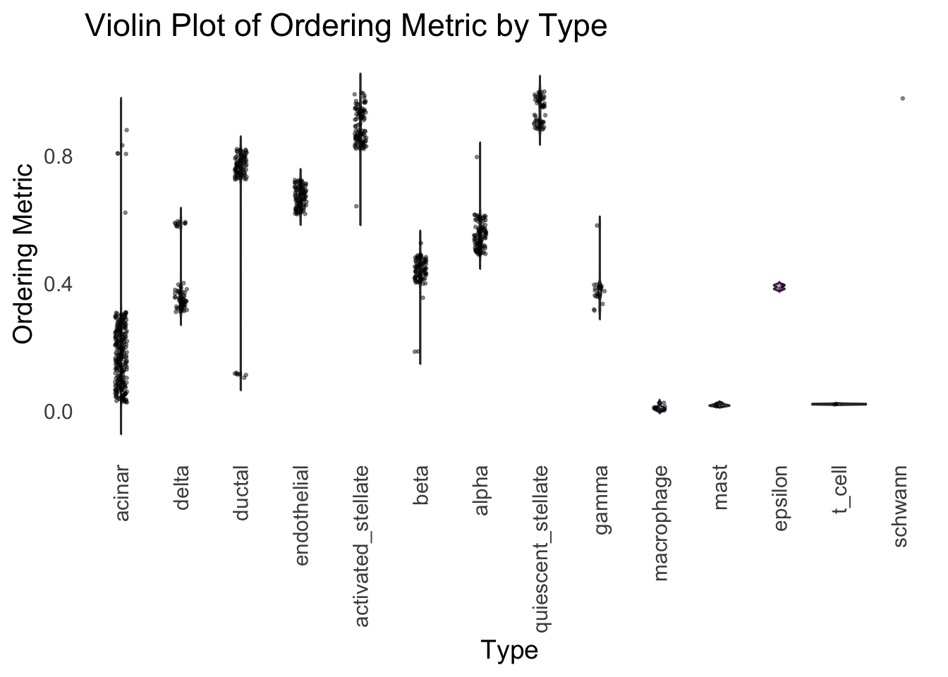

Past versions of unnamed-chunk-22-1.png

Version	Author	Date
2f5e139	Ziang Zhang	2025-07-08

Again, the hierarchical clustering ordering produces a clear separation between the cell types.

However, just like tSNE and UMAP, the hierarchical clustering ordering does not necessarily produce a interpretable global ordering structure. In particular, the ordering is not unique, as clades of the tree can be rearranged without changing the clustering result.

Ordering based on EM

Now, let’s try to obtain the ordering based on the smooth-EM algorithm.

Traditional EM

First, we will see how the traditional EM algorithm performs on the loadings.

library(mclust)

Package 'mclust' version 6.1.1
Type 'citation("mclust")' for citing this R package in publications.

fit_mclust <- Mclust(Loadings, G=100)

Let’s assume observations in the same cluster are ordered next to each other.

loadings_order_EM <- order(fit_mclust$classification)

plot_structure(Loadings, order = rownames(Loadings)[loadings_order_EM])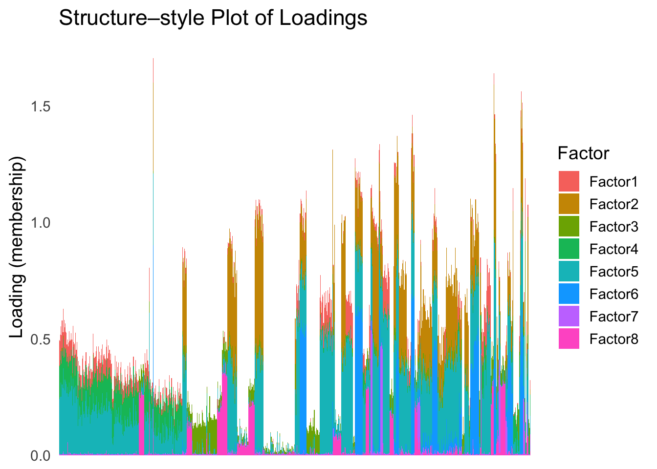

Past versions of unnamed-chunk-25-1.png

Version	Author	Date
29aee93	Ziang Zhang	2025-07-09

plot_highlight_types(type_vec = celltype,
                     subset_types = highlights,
                     order_vec = rownames(Loadings)[loadings_order_EM],
                     other_color = "white"
                     )

Past versions of unnamed-chunk-26-1.png

Version	Author	Date
29aee93	Ziang Zhang	2025-07-09

The same cell types tend to be clustered together, but the ordering does not make much sense. This is okay as we know in traditional EM, the index of the cluster is arbitrary.

Smooth-EM with linear prior

source("./code/linear_EM.R")
source("./code/general_EM.R")

Warning: package 'matrixStats' was built under R version 4.3.3

Warning: package 'mvtnorm' was built under R version 4.3.3

Attaching package: 'mvtnorm'

The following object is masked from 'package:mclust':

    dmvnorm

Attaching package: 'Matrix'

The following objects are masked from 'package:tidyr':

    expand, pack, unpack

source("./code/prior_precision.R")
result_linear <- EM_algorithm_linear(
  data = Loadings,
  K = 100,
  betaprec = 0.001,
  seed = 123,
  max_iter = 100,
  tol = 1e-3,
  verbose = TRUE
)

Iteration   1: objective = 7697.904951
Iteration   2: objective = 7707.333337
Iteration   3: objective = 7740.471790
Iteration   4: objective = 7824.680280
Iteration   5: objective = 7932.772390
Iteration   6: objective = 8004.887583
Iteration   7: objective = 8048.786905
Iteration   8: objective = 8082.151208
Iteration   9: objective = 8108.914531
Iteration  10: objective = 8128.262919
Iteration  11: objective = 8140.589009
Iteration  12: objective = 8148.242727
Iteration  13: objective = 8153.754444
Iteration  14: objective = 8158.892229
Iteration  15: objective = 8164.775036
Iteration  16: objective = 8172.209580
Iteration  17: objective = 8181.844606
Iteration  18: objective = 8194.050410
Iteration  19: objective = 8208.553655
Iteration  20: objective = 8224.115553
Iteration  21: objective = 8238.839898
Iteration  22: objective = 8251.246227
Iteration  23: objective = 8261.096431
Iteration  24: objective = 8269.093358
Iteration  25: objective = 8276.041121
Iteration  26: objective = 8282.391788
Iteration  27: objective = 8288.274436
Iteration  28: objective = 8293.675980
Iteration  29: objective = 8298.567980
Iteration  30: objective = 8302.950218
Iteration  31: objective = 8306.847980
Iteration  32: objective = 8310.299406
Iteration  33: objective = 8313.349138
Iteration  34: objective = 8316.047888
Iteration  35: objective = 8318.452196
Iteration  36: objective = 8320.621235
Iteration  37: objective = 8322.611615
Iteration  38: objective = 8324.472662
Iteration  39: objective = 8326.243878
Iteration  40: objective = 8327.954752
Iteration  41: objective = 8329.626164
Iteration  42: objective = 8331.272395
Iteration  43: objective = 8332.903070
Iteration  44: objective = 8334.524663
Iteration  45: objective = 8336.141525
Iteration  46: objective = 8337.756516
Iteration  47: objective = 8339.371381
Iteration  48: objective = 8340.986992
Iteration  49: objective = 8342.603518
Iteration  50: objective = 8344.220562
Iteration  51: objective = 8345.837262
Iteration  52: objective = 8347.452327
Iteration  53: objective = 8349.064049
Iteration  54: objective = 8350.670270
Iteration  55: objective = 8352.268358
Iteration  56: objective = 8353.855204
Iteration  57: objective = 8355.427242
Iteration  58: objective = 8356.980488
Iteration  59: objective = 8358.510581
Iteration  60: objective = 8360.012823
Iteration  61: objective = 8361.482229
Iteration  62: objective = 8362.913615
Iteration  63: objective = 8364.301750
Iteration  64: objective = 8365.641605
Iteration  65: objective = 8366.928691
Iteration  66: objective = 8368.159455
Iteration  67: objective = 8369.331684
Iteration  68: objective = 8370.444838
Iteration  69: objective = 8371.500247
Iteration  70: objective = 8372.501125
Iteration  71: objective = 8373.452390
Iteration  72: objective = 8374.360303
Iteration  73: objective = 8375.231997
Iteration  74: objective = 8376.074940
Iteration  75: objective = 8376.896412
Iteration  76: objective = 8377.703041
Iteration  77: objective = 8378.500430
Iteration  78: objective = 8379.292888
Iteration  79: objective = 8380.083277
Iteration  80: objective = 8380.872937
Iteration  81: objective = 8381.661719
Iteration  82: objective = 8382.448072
Iteration  83: objective = 8383.229208
Iteration  84: objective = 8384.001319
Iteration  85: objective = 8384.759839
Iteration  86: objective = 8385.499737
Iteration  87: objective = 8386.215835
Iteration  88: objective = 8386.903115
Iteration  89: objective = 8387.557006
Iteration  90: objective = 8388.173626
Iteration  91: objective = 8388.749967
Iteration  92: objective = 8389.284001
Iteration  93: objective = 8389.774717
Iteration  94: objective = 8390.222091
Iteration  95: objective = 8390.626991
Iteration  96: objective = 8390.991049
Iteration  97: objective = 8391.316501
Iteration  98: objective = 8391.606022
Iteration  99: objective = 8391.862565
Iteration 100: objective = 8392.089216

result_linear$clustering <- apply(result_linear$gamma, 1, which.max)
loadings_order_linear <- order(result_linear$clustering)
plot_structure(Loadings, order = rownames(Loadings)[loadings_order_linear])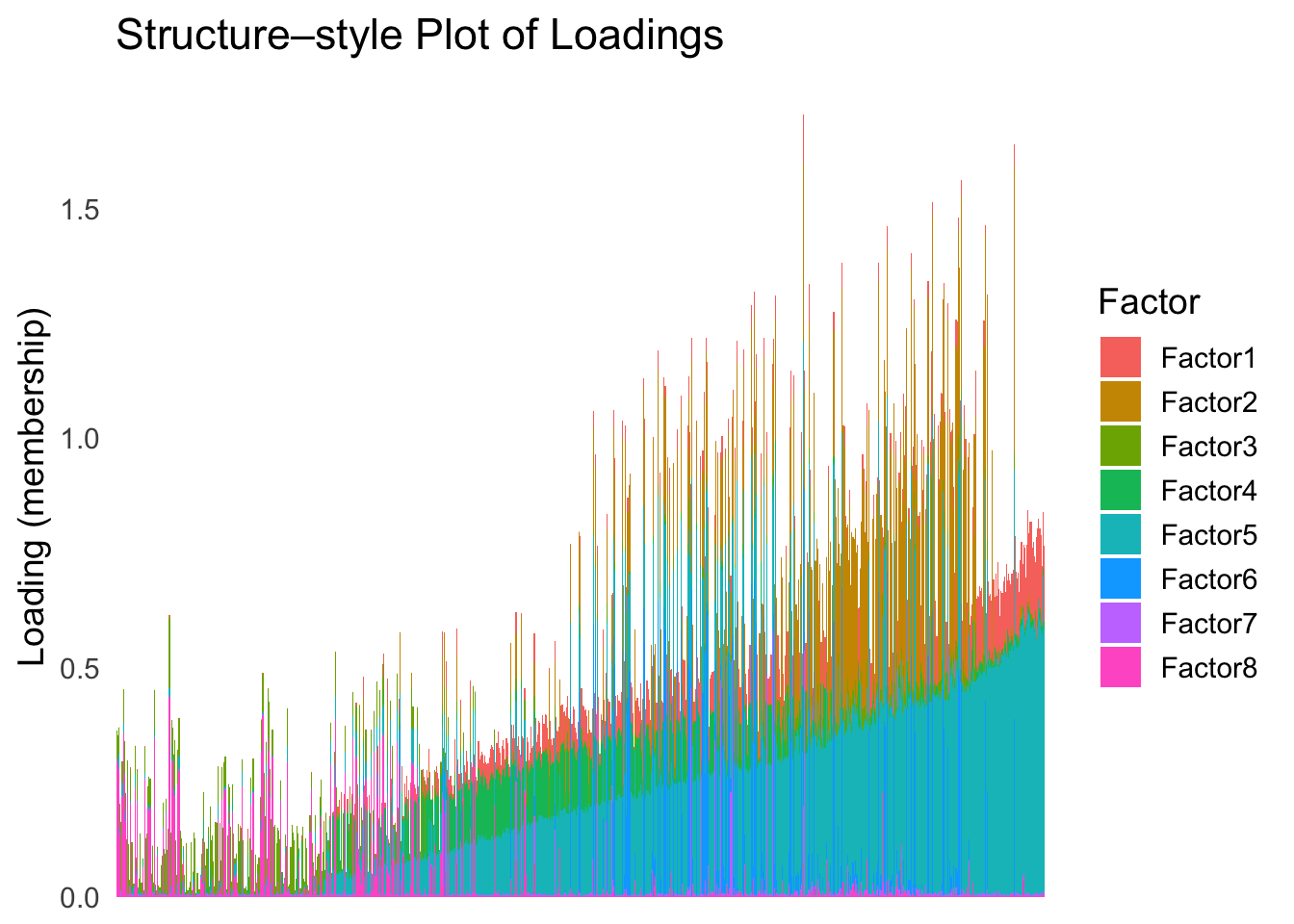

Past versions of unnamed-chunk-28-1.png

Version	Author	Date
29aee93	Ziang Zhang	2025-07-09

plot_highlight_types(type_vec = celltype,
                     subset_types = highlights,
                     order_vec = rownames(Loadings)[loadings_order_linear],
                     other_color = "white"
                     )

Past versions of unnamed-chunk-29-1.png

Version	Author	Date
29aee93	Ziang Zhang	2025-07-09

The ordering from linear prior does not look very informative, which is not unexpected since the linear prior is like a coarser version of the PCA.

Smooth-EM with RW1 prior

Now, let’s try the smooth-EM algorithm with a first order random walk prior.

set.seed(123)
Q_prior_RW1 <- make_random_walk_precision(K=100, d=ncol(Loadings), lambda = 10000, q=1)
init_params <- make_default_init(Loadings, K=100)
result_RW1 <- EM_algorithm(
  data = Loadings,
  Q_prior = Q_prior_RW1,
  init_params = init_params,
  max_iter = 100,
  modelName = "EEI",
  tol = 1e-3,
  verbose = TRUE
)

Iteration   1: objective = 11342.481336
Iteration   2: objective = 11342.492370
Iteration   3: objective = 11342.530363
Iteration   4: objective = 11342.714022
Iteration   5: objective = 11343.608347
Iteration   6: objective = 11347.901317
Iteration   7: objective = 11367.021400
Iteration   8: objective = 11433.676639
Iteration   9: objective = 11571.347654
Iteration  10: objective = 11747.174603
Iteration  11: objective = 12067.949655
Iteration  12: objective = 12788.480477
Iteration  13: objective = 14131.918367
Iteration  14: objective = 15061.694083
Iteration  15: objective = 15619.984311
Iteration  16: objective = 16199.798871
Iteration  17: objective = 16714.975200
Iteration  18: objective = 17142.303555
Iteration  19: objective = 17373.950565
Iteration  20: objective = 17426.934266
Iteration  21: objective = 17494.851962
Iteration  22: objective = 17526.820016
Iteration  23: objective = 17531.632651
Iteration  24: objective = 17545.615448
Iteration  25: objective = 17573.857249
Iteration  26: objective = 17576.728985
Iteration  27: objective = 17585.627075
Iteration  28: objective = 17590.942767
Iteration  29: objective = 17597.913291
Iteration  30: objective = 17597.418594
Converged at iteration 30 with objective 17597.418594

result_RW1$clustering <- apply(result_RW1$gamma, 1, which.max)
loadings_order_RW1 <- order(result_RW1$clustering)
plot_structure(Loadings, order = rownames(Loadings)[loadings_order_RW1])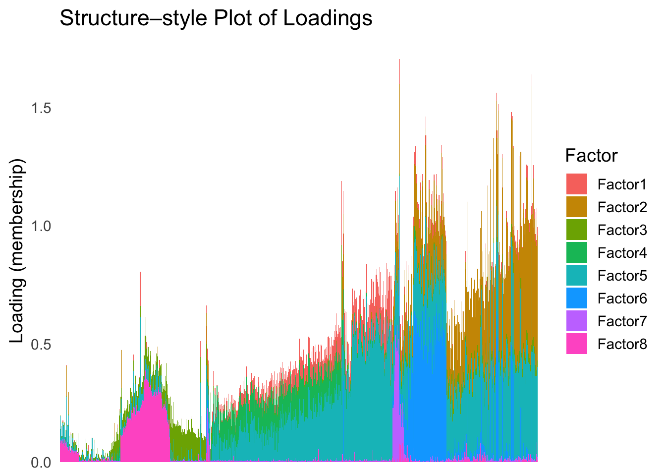

Past versions of unnamed-chunk-31-1.png

Version	Author	Date
29aee93	Ziang Zhang	2025-07-09

plot_highlight_types(type_vec = celltype,
                     subset_types = highlights,
                     order_vec = rownames(Loadings)[loadings_order_RW1],
                     other_color = "white"
                     )

Past versions of unnamed-chunk-32-1.png

Version	Author	Date
29aee93	Ziang Zhang	2025-07-09

The result from RW1 looks good. Each cell type is separated from the others, and the ordering seems to make sense.

Smooth-EM with RW2 prior

Next, we will try the RW2 prior in the smooth-EM algorithm.

Q_prior_RW2 <- make_random_walk_precision(K=100, d=ncol(Loadings), lambda = 20000, q=2)
set.seed(1234)
init_params <- make_default_init(Loadings, K=100)
result_RW2 <- EM_algorithm(
  data = Loadings,
  Q_prior = Q_prior_RW2,
  init_params = init_params,
  max_iter = 100,
  modelName = "EEI",
  tol = 1e-3,
  verbose = TRUE
)

Iteration   1: objective = 11610.707865
Iteration   2: objective = 11611.012288
Iteration   3: objective = 11612.467725
Iteration   4: objective = 11619.537033
Iteration   5: objective = 11651.133683
Iteration   6: objective = 11763.143096
Iteration   7: objective = 12019.538719
Iteration   8: objective = 12406.384211
Iteration   9: objective = 13195.240188
Iteration  10: objective = 14797.093833
Iteration  11: objective = 16171.899758
Iteration  12: objective = 17359.843511
Iteration  13: objective = 18397.170248
Iteration  14: objective = 18788.820493
Iteration  15: objective = 18927.026536
Iteration  16: objective = 18983.743391
Iteration  17: objective = 19002.218344
Iteration  18: objective = 18976.113164
Converged at iteration 18 with objective 18976.113164

result_RW2$clustering <- apply(result_RW2$gamma, 1, which.max)
loadings_order_RW2 <- order(result_RW2$clustering)
plot_structure(Loadings, order = rownames(Loadings)[loadings_order_RW2])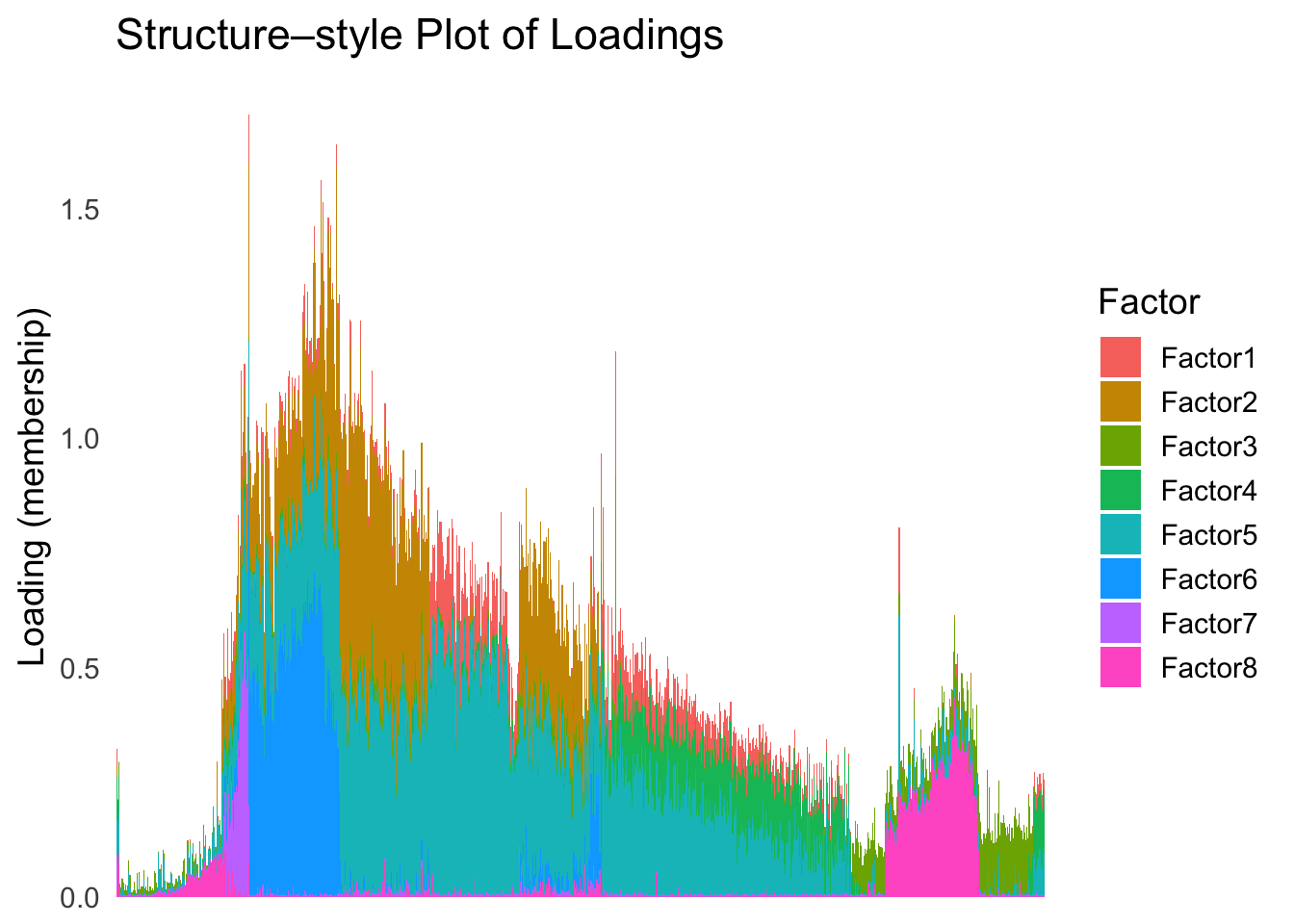

Past versions of unnamed-chunk-34-1.png

Version	Author	Date
29aee93	Ziang Zhang	2025-07-09

plot_highlight_types(type_vec = celltype,
                     subset_types = highlights,
                     order_vec = rownames(Loadings)[loadings_order_RW2],
                     other_color = "white"
                     )

Past versions of unnamed-chunk-35-1.png

Version	Author	Date
29aee93	Ziang Zhang	2025-07-09

The result also looks good, but the choice of the smoothing parameter (lambda) is very important…

Session information

sessionInfo()

R version 4.3.1 (2023-06-16)
Platform: aarch64-apple-darwin20 (64-bit)
Running under: macOS Monterey 12.7.4

Matrix products: default
BLAS:   /Library/Frameworks/R.framework/Versions/4.3-arm64/Resources/lib/libRblas.0.dylib 
LAPACK: /Library/Frameworks/R.framework/Versions/4.3-arm64/Resources/lib/libRlapack.dylib;  LAPACK version 3.11.0

locale:
[1] en_US.UTF-8/en_US.UTF-8/en_US.UTF-8/C/en_US.UTF-8/en_US.UTF-8

time zone: America/Chicago
tzcode source: internal

attached base packages:
[1] stats     graphics  grDevices utils     datasets  methods   base     

other attached packages:
 [1] Matrix_1.6-4      mvtnorm_1.3-1     matrixStats_1.4.1 mclust_6.1.1     
 [5] umap_0.2.10.0     Rtsne_0.17        ggplot2_3.5.2     tidyr_1.3.1      
 [9] tibble_3.2.1      workflowr_1.7.1  

loaded via a namespace (and not attached):
 [1] sass_0.4.10        generics_0.1.4     stringi_1.8.7      lattice_0.22-6    
 [5] digest_0.6.37      magrittr_2.0.3     evaluate_1.0.3     grid_4.3.1        
 [9] RColorBrewer_1.1-3 fastmap_1.2.0      rprojroot_2.0.4    jsonlite_2.0.0    
[13] processx_3.8.6     whisker_0.4.1      RSpectra_0.16-2    ps_1.9.1          
[17] promises_1.3.3     httr_1.4.7         purrr_1.0.4        scales_1.4.0      
[21] jquerylib_0.1.4    cli_3.6.5          rlang_1.1.6        withr_3.0.2       
[25] cachem_1.1.0       yaml_2.3.10        tools_4.3.1        dplyr_1.1.4       
[29] httpuv_1.6.16      reticulate_1.42.0  png_0.1-8          vctrs_0.6.5       
[33] R6_2.6.1           lifecycle_1.0.4    git2r_0.33.0       stringr_1.5.1     
[37] fs_1.6.6           pkgconfig_2.0.3    callr_3.7.6        pillar_1.10.2     
[41] bslib_0.9.0        later_1.4.2        gtable_0.3.6       glue_1.8.0        
[45] Rcpp_1.0.14        xfun_0.52          tidyselect_1.2.1   rstudioapi_0.16.0 
[49] knitr_1.50         farver_2.1.2       htmltools_0.5.8.1  labeling_0.4.3    
[53] rmarkdown_2.28     compiler_4.3.1     getPass_0.2-4      askpass_1.2.1     
[57] openssl_2.2.2