Explore Complex Posterior Functions

workflowr

• Summary
• Checks
• Past versions

Last updated: 2025-04-24

Checks: 7 0

Knit directory: BOSS_website/

This reproducible R Markdown analysis was created with workflowr (version 1.7.1). The Checks tab describes the reproducibility checks that were applied when the results were created. The Past versions tab lists the development history.

---

R Markdown file: up-to-date

Great! Since the R Markdown file has been committed to the Git repository, you know the exact version of the code that produced these results.

Environment: empty

Great job! The global environment was empty. Objects defined in the global environment can affect the analysis in your R Markdown file in unknown ways. For reproduciblity it’s best to always run the code in an empty environment.

Seed: set.seed(20250415)

The command set.seed(20250415) was run prior to running the code in the R Markdown file. Setting a seed ensures that any results that rely on randomness, e.g. subsampling or permutations, are reproducible.

Session information: recorded

Great job! Recording the operating system, R version, and package versions is critical for reproducibility.

Cache: none

Nice! There were no cached chunks for this analysis, so you can be confident that you successfully produced the results during this run.

File paths: relative

Great job! Using relative paths to the files within your workflowr project makes it easier to run your code on other machines.

Repository version: 9d2ee8c

Great! You are using Git for version control. Tracking code development and connecting the code version to the results is critical for reproducibility.

The results in this page were generated with repository version 9d2ee8c. See the Past versions tab to see a history of the changes made to the R Markdown and HTML files.

Note that you need to be careful to ensure that all relevant files for the analysis have been committed to Git prior to generating the results (you can use wflow_publish or wflow_git_commit). workflowr only checks the R Markdown file, but you know if there are other scripts or data files that it depends on. Below is the status of the Git repository when the results were generated:

Ignored files:
    Ignored:    .DS_Store
    Ignored:    .Rhistory
    Ignored:    .Rproj.user/
    Ignored:    analysis/.DS_Store
    Ignored:    analysis/.Rhistory
    Ignored:    code/.DS_Store
    Ignored:    data/.DS_Store
    Ignored:    data/sim1/
    Ignored:    output/.DS_Store
    Ignored:    output/sim2/.DS_Store

Untracked files:
    Untracked:  code/mortality_BG_grid.R
    Untracked:  code/mortality_NL_grid.R
    Untracked:  data/co2/
    Untracked:  data/mortality/
    Untracked:  data/simA1/
    Untracked:  output/co2/
    Untracked:  output/mortality/
    Untracked:  output/sim2/quad_sparse_list.rda
    Untracked:  output/simA1/

Unstaged changes:
    Modified:   output/sim2/BO_data_to_smooth.rda
    Modified:   output/sim2/BO_result_list.rda
    Modified:   output/sim2/rel_runtime.rda

Note that any generated files, e.g. HTML, png, CSS, etc., are not included in this status report because it is ok for generated content to have uncommitted changes.

---

These are the previous versions of the repository in which changes were made to the R Markdown (analysis/simA1.Rmd) and HTML (docs/simA1.html) files. If you’ve configured a remote Git repository (see ?wflow_git_remote), click on the hyperlinks in the table below to view the files as they were in that past version.

File	Version	Author	Date	Message
Rmd	9d2ee8c	Ziang Zhang	2025-04-24	workflowr::wflow_publish("analysis/simA1.Rmd")
Rmd	325128f	Ziang Zhang	2025-04-22	Update BOSS function
html	ff55aef	Ziang Zhang	2025-04-21	Build site.
Rmd	2bcc0e0	Ziang Zhang	2025-04-21	workflowr::wflow_publish("analysis/simA1.Rmd")
html	d35a475	Ziang Zhang	2025-04-21	Build site.
Rmd	a593785	Ziang Zhang	2025-04-21	workflowr::wflow_publish("analysis/simA1.Rmd")

---

Introduction

In this example, we assess the accuracy of the proposed BOSS algorithm for approximating (un-normalized) posterior functions with different complexities.

We consider a conditioning parameter \(\alpha\) with support \(\Omega = [0,10]\), and assume its unnormalized log posteriors are defined respectively as \(f(\alpha) = \alpha \sin(\alpha)\), \(\log(\alpha+1)\sin(2\alpha) - \alpha \cos(2\alpha)\), and \(\log(\alpha + 1) (\sin(4\alpha) + \cos(2\alpha))\) for simple, medium, and hard settings.

In the simple setting, the log posterior has two local modes and its corresponding posterior is close to uni-modal. In the medium scenario, the log posterior has three local modes, with the corresponding posterior that is close to bi-modal. In the hard scenario, the log posterior has seven local modes and the posterior is close to tri-modal. The proposed BOSS algorithm is then applied with different numbers of BO iterations \(B\) with five initial values that are equally placed from 0 to 10.

library(npreg)

Package 'npreg' version 1.1.0
Type 'citation("npreg")' to cite this package.

library(ggplot2)
library(aghq)

set.seed(123)
noise_var = 1e-6
function_path <- "./code"
output_path <- "./output/simA1"
data_path <- "./data/simA1"
source(paste0(function_path, "/00_BOSS.R"))

surrogate <- function(xvalue, data_to_smooth){
  predict(ss(x = as.numeric(data_to_smooth$x), y = data_to_smooth$y, df = length(unique(as.numeric(data_to_smooth$x))), m = 2, all.knots = TRUE), x = xvalue)$y
}
lower = 0
upper = 10

integrate_aghq <- function(f, k = 100, startingvalue = 0){
  ff <- list(fn = f, gr = function(x) numDeriv::grad(f, x), he = function(x) numDeriv::hessian(f, x))
  aghq(ff = ff, k = k, startingvalue = startingvalue)$normalized_posterior$lognormconst
}

#### Compute the KL distance:
Compute_KL <- function(x, logpx, logqx){
  dx <- diff(x)
  left <- c(0,dx)
  right <- c(dx,0)
  0.5 * sum(left * (logpx - logqx) * exp(logpx)) + 0.5 * sum(right * (logpx - logqx) * exp(logpx))
}

#### Compute the KS distance:
Compute_KS <- function(x, qx, px){
  dx <- c(diff(x),0)
  max(abs(cumsum(qx * dx) - cumsum(px * dx)))
}

Easy Example:

Define the log posterior function:

log_prior <- function(x){
  1
}
log_likelihood <- function(x){
  x*sin(x)
}
eval_once <- function(x){
  log_prior(x) + log_likelihood(x)
}
eval_once_mapped <- function(y){
  eval_once(pnorm(y) * (upper - lower) + lower) + dnorm(y, log = T) + log(upper - lower)
}
x <- seq(0.01,9.99, by = 0.01)
y <- qnorm((x - lower)/(upper - lower))
true_log_norm_constant <- integrate_aghq(f = function(y) eval_once_mapped(y))
true_log_post_mapped <- function(y) {eval_once_mapped(y) - true_log_norm_constant}
plot((true_log_post_mapped(y)) ~ y, type = "l", cex.lab = 1.5, cex.axis = 1.5, 
     xlab = "y", ylab = "log density", lwd = 2, col = "blue")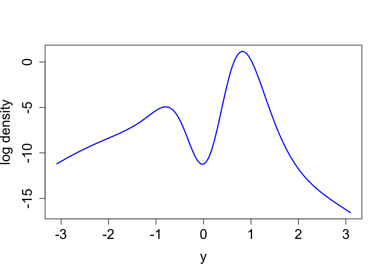

Past versions of unnamed-chunk-2-1.png

Version	Author	Date
d35a475	Ziang Zhang	2025-04-21

true_log_post <- function(x) {true_log_post_mapped(qnorm((x - lower)/(upper - lower))) - dnorm(qnorm((x - lower)/(upper - lower)), log = T) - log(upper - lower)}
integrate(function(x) exp(true_log_post(x)), lower = 0, upper = 10)

1.000275 with absolute error < 9.7e-05

Let’s run BOSS with the above log posterior function:

objective_func <- eval_once
eval_num <- seq(5, 100, by = 5)

result_ad <- BOSS(
  func = eval_once, initial_design = 5,
  update_step = 5, max_iter = (max(eval_num) - 5),
  opt.lengthscale.grid = 100, opt.grid = 1000,
  delta = 0.01, noise_var = noise_var,
  lower = lower, upper = upper,
  verbose = 0,
  modal_iter_check = 5, modal_check_warmup = 10, modal_k.nn = 5, modal_eps = 0, criterion = "modal"
)
saveRDS(result_ad, file = paste0(data_path, "/result_ad_easy.rds"))

BO_result_list <- list()
BO_result_original_list <- list()
result_ad <- readRDS(file = paste0(data_path, "/result_ad_easy.rds"))
for (i in 1:length(eval_num)) {
  eval_number <- eval_num[i]

  result_ad_selected <- list(x = result_ad$result$x[1:eval_number, ],
                             x_original = result_ad$result$x_original[1:eval_number, ],
                             y = result_ad$result$y[1:eval_number])
  
  data_to_smooth <- result_ad_selected
  BO_result_original_list[[i]] <- data_to_smooth

  ff <- list()
  ff$fn <- function(y) as.numeric(surrogate(pnorm(y), data_to_smooth = data_to_smooth) + dnorm(y, log = TRUE))
  fn_vals <- sapply(y, ff$fn)

  lognormal_const <- integrate_aghq(f = ff$fn)
  post_y <- data.frame(y = y, pos = exp(fn_vals - lognormal_const))
  post_x <- data.frame(x = pnorm(post_y$y) * (upper - lower) + lower, post = (post_y$pos / dnorm(post_y$y))/(upper - lower) )
  
  BO_result_list[[i]] <- post_x
}
saveRDS(BO_result_list, file = paste0(data_path, "/BO_result_list_easy.rds"))
saveRDS(BO_result_original_list, file = paste0(data_path, "/BO_result_original_list_easy.rds"))

Some illustrations

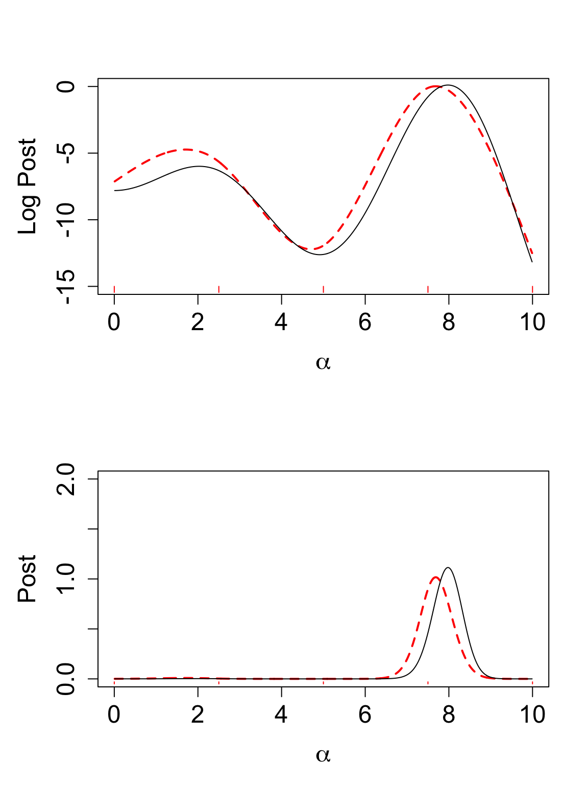
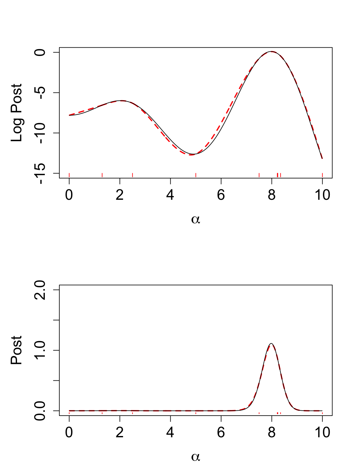
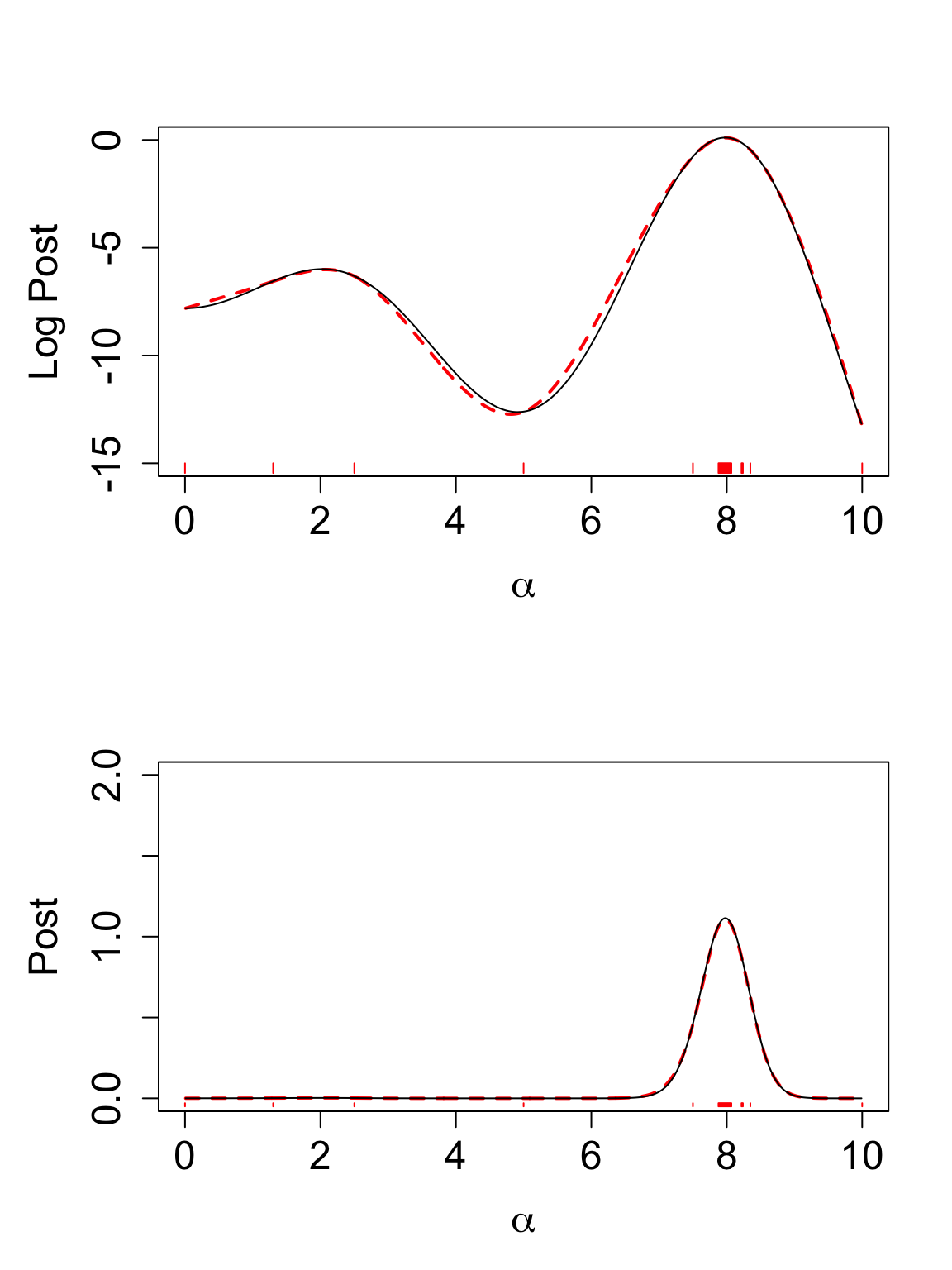
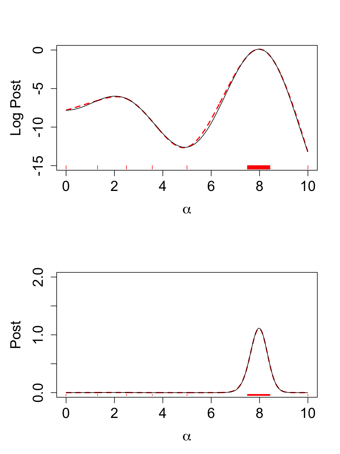
Here are some illustrations of the approximated posterior from BOSS with different numbers of BO iterations \(B\) (red: approximated posterior, black: true posterior).

BO_result_list <- readRDS(file = paste0(data_path, "/BO_result_list_easy.rds"))
BO_result_original_list <- readRDS(file = paste0(data_path, "/BO_result_original_list_easy.rds"))

B = 5

to_plot_data <- BO_result_list[[1]]
to_plot_data$logpos <- log(to_plot_data$pos)
to_plot_data_obs <- BO_result_original_list[[1]]
y_min <- -15; y_max <- 0
mar.default <- c(5,4,4,2)
par(mar = mar.default + c(0, 1, 0, 0), mfrow = c(2, 1))
plot(to_plot_data$logpos ~ to_plot_data$x, 
       type = "l", lty = "dashed", col = "red", lwd = 2,
       ylab = "Log Post", xlab = expression(alpha),
       ylim = c(y_min, y_max), cex.lab = 1.5, cex.axis = 1.5)
lines((true_log_post(x)) ~ x, lwd = 1)
y_offset <- 0.03 * (y_max - y_min) # adjust offset as needed
for(x_val in to_plot_data_obs$x_original) {
    segments(x_val, y_min, x_val, y_min - y_offset, col = "red")
}

plot(exp(to_plot_data$logpos) ~ to_plot_data$x, 
       type = "l", lty = "dashed", col = "red", lwd = 2,
       ylab = "Post", xlab = expression(alpha), ylim = c(0,2), cex.lab = 1.5, cex.axis = 1.5)
lines(exp(true_log_post(x)) ~ x, lwd = 1)
y_min <- -0.03
y_offset <- 0.01 * (2) # adjust offset as needed
for(x_val in to_plot_data_obs$x_original) {
    segments(x_val, y_min, x_val, y_min - y_offset, col = "red")
}

Past versions of unnamed-chunk-7-1.png

Version	Author	Date
d35a475	Ziang Zhang	2025-04-21

B = 10

to_plot_data <- BO_result_list[[2]]
to_plot_data$logpos <- log(to_plot_data$pos)
to_plot_data_obs <- BO_result_original_list[[2]]
y_min <- -15; y_max <- 0

mar.default <- c(5,4,4,2)
par(mar = mar.default + c(0, 1, 0, 0), mfrow = c(2, 1))
plot(to_plot_data$logpos ~ to_plot_data$x, 
       type = "l", lty = "dashed", col = "red", lwd = 2,
       ylab = "Log Post", xlab = expression(alpha),
       ylim = c(y_min, y_max), cex.lab = 1.5, cex.axis = 1.5)
lines((true_log_post(x)) ~ x, lwd = 1)
y_offset <- 0.03 * (y_max - y_min) # adjust offset as needed
for(x_val in to_plot_data_obs$x_original) {
    segments(x_val, y_min, x_val, y_min - y_offset, col = "red")
}

plot(exp(to_plot_data$logpos) ~ to_plot_data$x, 
       type = "l", lty = "dashed", col = "red", lwd = 2,
       ylab = "Post", xlab = expression(alpha), ylim = c(0,2), cex.lab = 1.5, cex.axis = 1.5)
lines(exp(true_log_post(x)) ~ x, lwd = 1)
y_min <- -0.03
y_offset <- 0.01 * (2) # adjust offset as needed
for(x_val in to_plot_data_obs$x_original) {
    segments(x_val, y_min, x_val, y_min - y_offset, col = "red")
}

Past versions of unnamed-chunk-8-1.png

Version	Author	Date
d35a475	Ziang Zhang	2025-04-21

B = 30

to_plot_data <- BO_result_list[[6]]
to_plot_data$logpos <- log(to_plot_data$pos)
to_plot_data_obs <- BO_result_original_list[[6]]
y_min <- -15; y_max <- 0

mar.default <- c(5,4,4,2)
par(mar = mar.default + c(0, 1, 0, 0), mfrow = c(2, 1))
plot(to_plot_data$logpos ~ to_plot_data$x, 
       type = "l", lty = "dashed", col = "red", lwd = 2,
       ylab = "Log Post", xlab = expression(alpha),
       ylim = c(y_min, y_max), cex.lab = 1.5, cex.axis = 1.5)
lines((true_log_post(x)) ~ x, lwd = 1)
y_offset <- 0.03 * (y_max - y_min) # adjust offset as needed
for(x_val in to_plot_data_obs$x_original) {
    segments(x_val, y_min, x_val, y_min - y_offset, col = "red")
}

plot(exp(to_plot_data$logpos) ~ to_plot_data$x, 
       type = "l", lty = "dashed", col = "red", lwd = 2,
       ylab = "Post", xlab = expression(alpha), ylim = c(0,2), cex.lab = 1.5, cex.axis = 1.5)
lines(exp(true_log_post(x)) ~ x, lwd = 1)
y_min <- -0.03
y_offset <- 0.01 * (2) # adjust offset as needed
for(x_val in to_plot_data_obs$x_original) {
    segments(x_val, y_min, x_val, y_min - y_offset, col = "red")
}

Past versions of unnamed-chunk-9-1.png

Version	Author	Date
d35a475	Ziang Zhang	2025-04-21

B = 100

to_plot_data <- BO_result_list[[20]]
to_plot_data$logpos <- log(to_plot_data$pos)
to_plot_data_obs <- BO_result_original_list[[20]]
y_min <- -15; y_max <- 0

mar.default <- c(5,4,4,2)
par(mar = mar.default + c(0, 1, 0, 0), mfrow = c(2, 1))
plot(to_plot_data$logpos ~ to_plot_data$x, 
       type = "l", lty = "dashed", col = "red", lwd = 2,
       ylab = "Log Post", xlab = expression(alpha),
       ylim = c(y_min, y_max), cex.lab = 1.5, cex.axis = 1.5)
lines((true_log_post(x)) ~ x, lwd = 1)
y_offset <- 0.03 * (y_max - y_min) # adjust offset as needed
for(x_val in to_plot_data_obs$x_original) {
    segments(x_val, y_min, x_val, y_min - y_offset, col = "red")
}

plot(exp(to_plot_data$logpos) ~ to_plot_data$x, 
       type = "l", lty = "dashed", col = "red", lwd = 2,
       ylab = "Post", xlab = expression(alpha), ylim = c(0,2), cex.lab = 1.5, cex.axis = 1.5)
lines(exp(true_log_post(x)) ~ x, lwd = 1)
y_min <- -0.03
y_offset <- 0.01 * (2) # adjust offset as needed
for(x_val in to_plot_data_obs$x_original) {
    segments(x_val, y_min, x_val, y_min - y_offset, col = "red")
}

Past versions of unnamed-chunk-10-1.png

Version	Author	Date
d35a475	Ziang Zhang	2025-04-21

KL and KS:

Let’s visualize the KL and KS divergence between the true posterior and the approximated posterior from BOSS.

KL_vec <- c()
for (i in 1:length(eval_num)) {
  KL_vec[i] <- Compute_KL(x = x, logpx = true_log_post(x), logqx = log(BO_result_list[[i]]$pos))
}
mar.default <- c(5,4,4,2)
par(mar = mar.default + c(0, 1, 0, 0))
plot((KL_vec) ~ eval_num, type = "o", ylab = "KL", xlab = "eval number: B", cex.lab = 1.5, cex.axis = 1.5)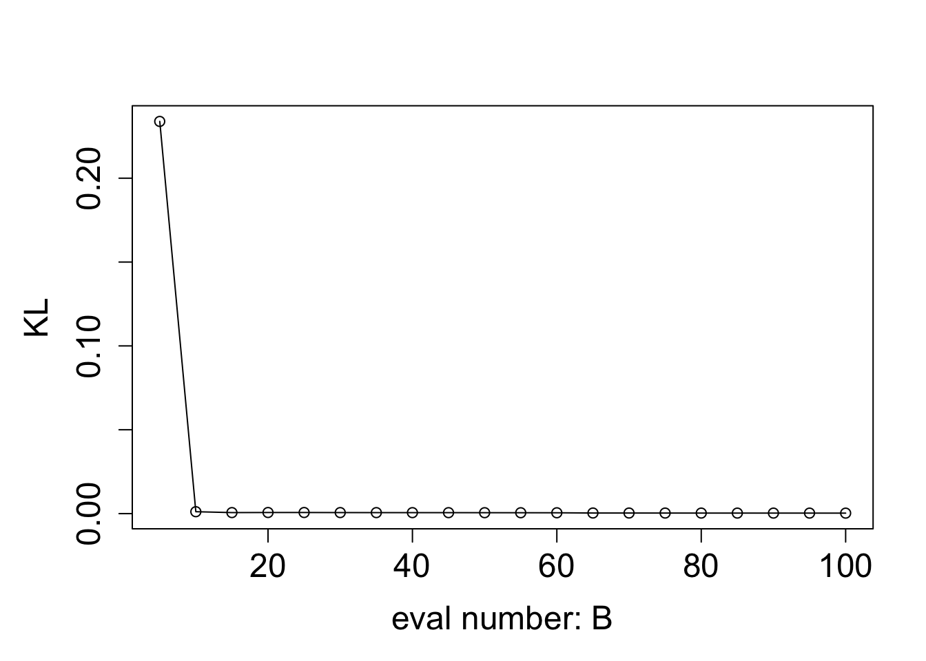

KS_vec <- c()
for (i in 1:length(eval_num)) {
  KS_vec[i] <- Compute_KS(x = x, px = exp(true_log_post(x)), qx = BO_result_list[[i]]$pos)
}
mar.default <- c(5,4,4,2)
par(mar = mar.default + c(0, 1, 0, 0))
plot((KS_vec) ~ eval_num, type = "o", ylab = "KS", xlab = "eval number: B", ylim = c(0,1), cex.lab = 1.5, cex.axis = 1.5)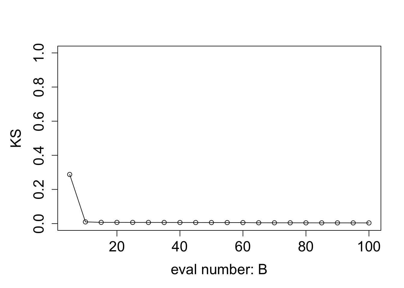

Based on the KL and KS divergence, we can the approximated posterior from BOSS is indistinguishable from the true posterior after 10 iterations in the simple example.

Medium Example:

Define the log posterior function:

log_prior <- function(x){
  1
}
log_likelihood <- function(x){
  log(x+1)*sin(x*2) - x*cos(x*2)
}
eval_once <- function(x){
  log_prior(x) + log_likelihood(x)
}
eval_once_mapped <- function(y){
  eval_once(pnorm(y) * (upper - lower) + lower) + dnorm(y, log = T) + log(upper - lower)
}
x <- seq(0.01,9.99, by = 0.01)
y <- qnorm((x - lower)/(upper - lower))
true_log_norm_constant <- integrate_aghq(f = function(y) eval_once_mapped(y), k = 100)
true_log_post_mapped <- function(y) {eval_once_mapped(y) - true_log_norm_constant}
plot((true_log_post_mapped(y)) ~ y, type = "l", cex.lab = 1.5, cex.axis = 1.5, 
     xlab = "y", ylab = "log density", lwd = 2, col = "blue")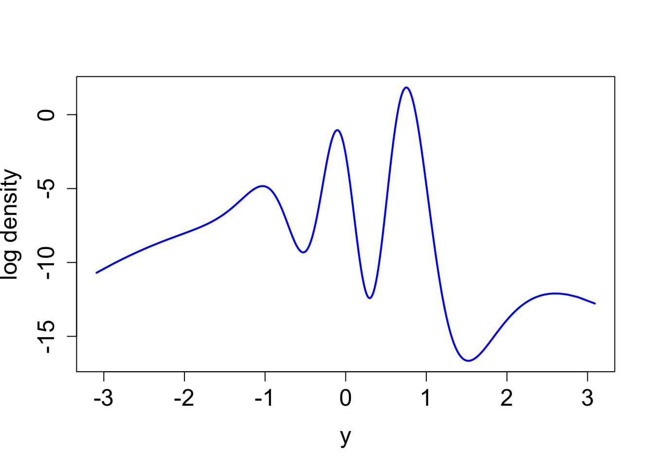

Past versions of unnamed-chunk-14-1.png

Version	Author	Date
d35a475	Ziang Zhang	2025-04-21

true_log_post <- function(x) {true_log_post_mapped(qnorm((x - lower)/(upper - lower))) - dnorm(qnorm((x - lower)/(upper - lower)), log = T) - log(upper - lower)}
integrate(function(x) exp(true_log_post(x)), lower = 0, upper = 10)

1.001231 with absolute error < 2.3e-05

Let’s run BOSS with the above log posterior function:

objective_func <- eval_once

result_ad <- BOSS(
  func = objective_func, initial_design = 5,
  update_step = 5, max_iter = (max(eval_num) - 5),
  opt.lengthscale.grid = 100, opt.grid = 1000,
  delta = 0.01, noise_var = noise_var,
  lower = lower, upper = upper,
  modal_iter_check = 5, modal_check_warmup = 10, modal_k.nn = 5, modal_eps = 0, criterion = "modal"
)
saveRDS(result_ad, file = paste0(data_path, "/result_ad_med.rds"))

BO_result_list <- list()
BO_result_original_list <- list()
result_ad <- readRDS(file = paste0(data_path, "/result_ad_med.rds"))
for (i in 1:length(eval_num)) {
  eval_number <- eval_num[i]

  result_ad_selected <- list(x = result_ad$result$x[1:eval_number, ],
                             x_original = result_ad$result$x_original[1:eval_number, ],
                             y = result_ad$result$y[1:eval_number])
  
  data_to_smooth <- result_ad_selected
  BO_result_original_list[[i]] <- data_to_smooth

  ff <- list()
  ff$fn <- function(y) as.numeric(surrogate(pnorm(y), data_to_smooth = data_to_smooth) + dnorm(y, log = TRUE))
  fn_vals <- sapply(y, ff$fn)

  lognormal_const <- integrate_aghq(f = ff$fn)
  post_y <- data.frame(y = y, pos = exp(fn_vals - lognormal_const))
  post_x <- data.frame(x = pnorm(post_y$y) * (upper - lower) + lower, post = (post_y$pos / dnorm(post_y$y))/(upper - lower) )
  
  BO_result_list[[i]] <- post_x
}
saveRDS(BO_result_list, file = paste0(data_path, "/BO_result_list_med.rds"))
saveRDS(BO_result_original_list, file = paste0(data_path, "/BO_result_original_list_med.rds"))

Some illustrations

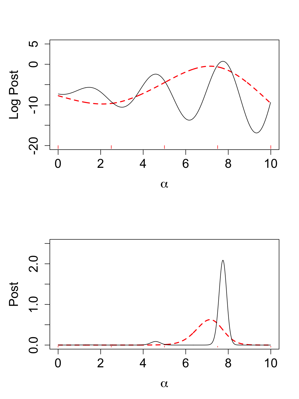
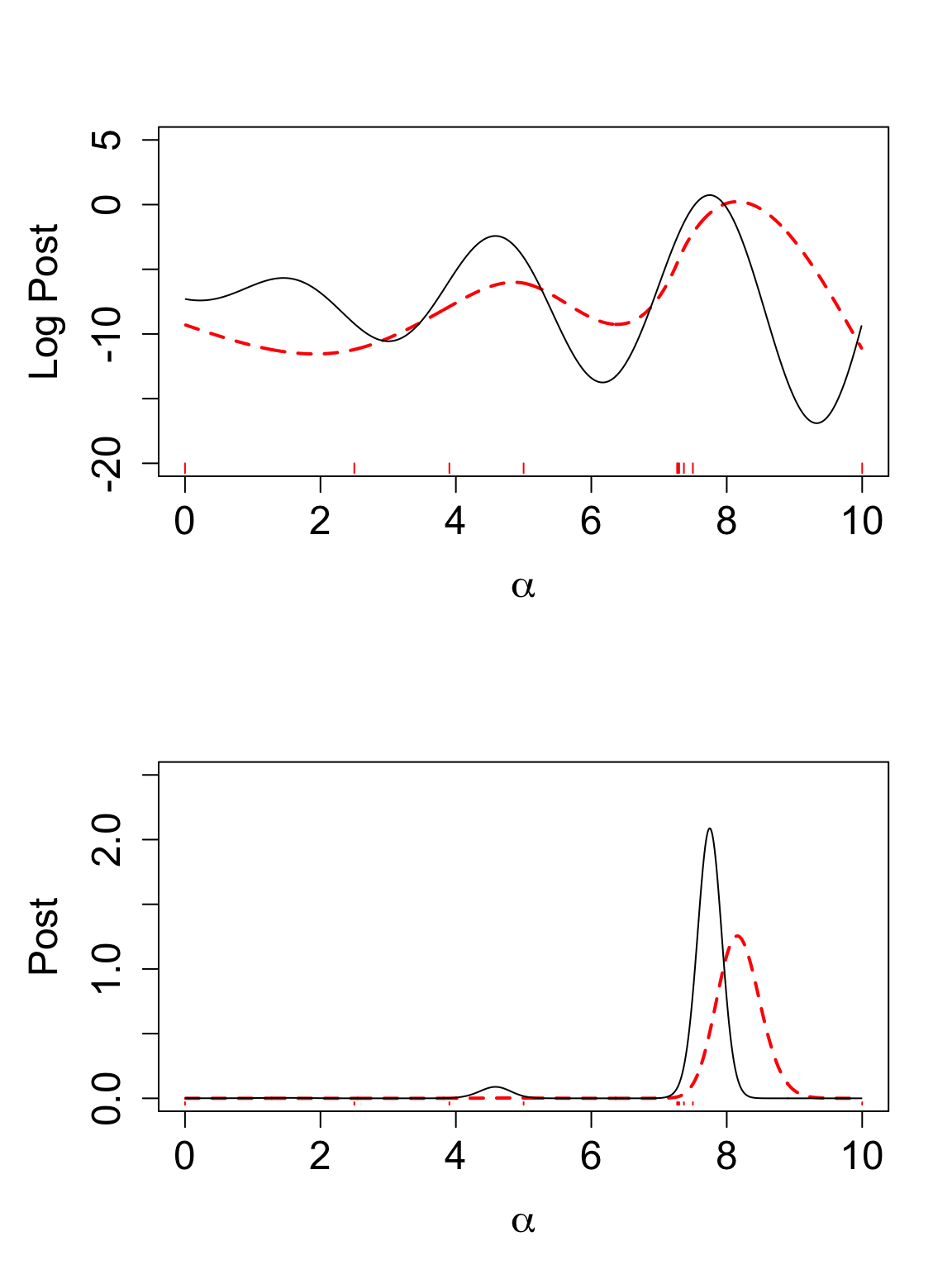
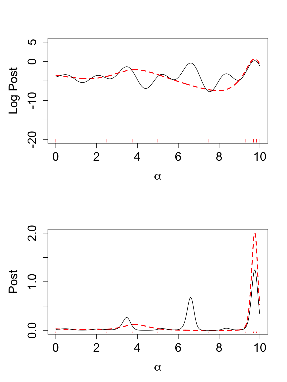
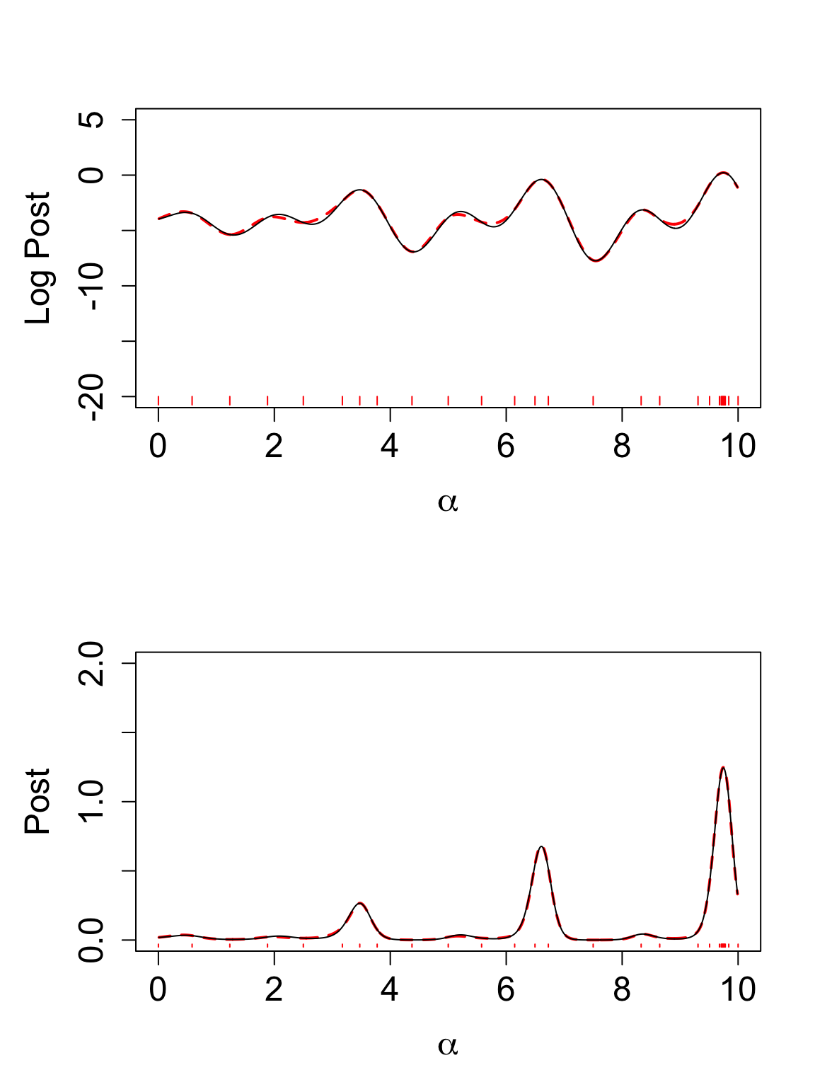
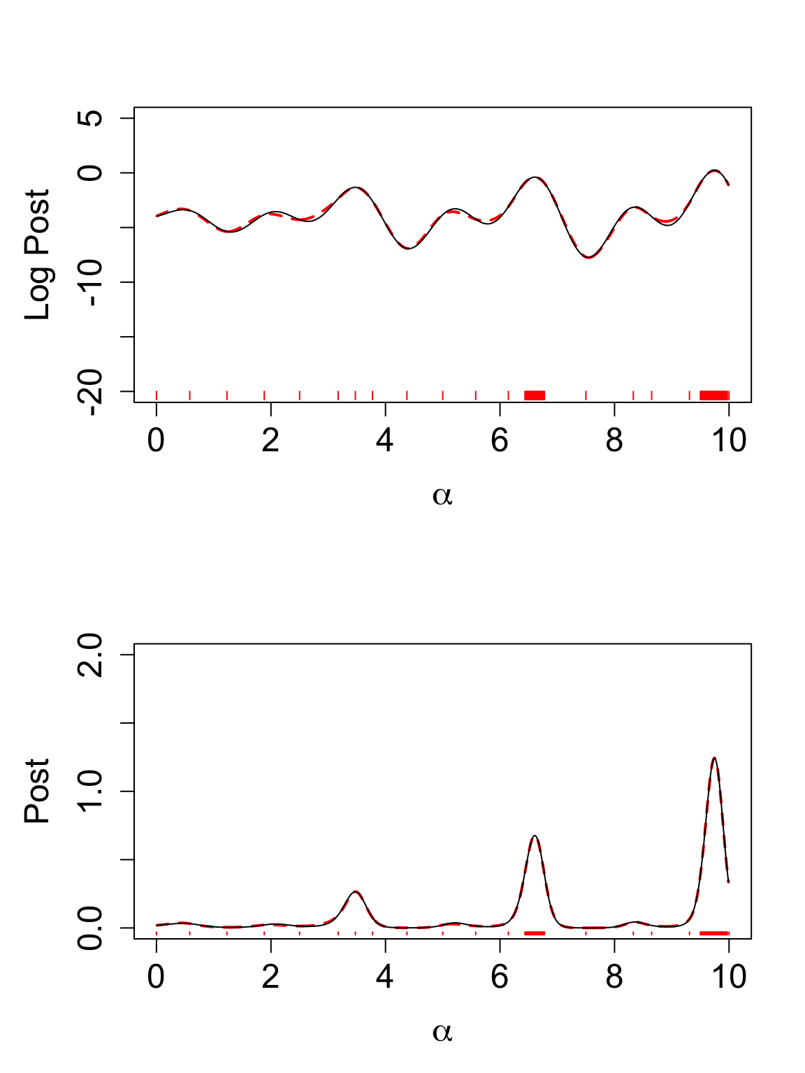
Here are some illustrations of the approximated posterior from BOSS with different numbers of BO iterations \(B\) (red: approximated posterior, black: true posterior).

BO_result_list <- readRDS(file = paste0(data_path, "/BO_result_list_med.rds"))
BO_result_original_list <- readRDS(file = paste0(data_path, "/BO_result_original_list_med.rds"))

B = 5

to_plot_data <- BO_result_list[[1]]
to_plot_data$logpos <- log(to_plot_data$pos)
to_plot_data_obs <- BO_result_original_list[[1]]
y_min <- -20; y_max <- 5
mar.default <- c(5,4,4,2)
par(mar = mar.default + c(0, 1, 0, 0), mfrow = c(2, 1))
plot(to_plot_data$logpos ~ to_plot_data$x, 
       type = "l", lty = "dashed", col = "red", lwd = 2,
       ylab = "Log Post", xlab = expression(alpha),
       ylim = c(y_min, y_max), cex.lab = 1.5, cex.axis = 1.5)
lines((true_log_post(x)) ~ x, lwd = 1)
y_offset <- 0.03 * (y_max - y_min) # adjust offset as needed
for(x_val in to_plot_data_obs$x_original) {
    segments(x_val, y_min, x_val, y_min - y_offset, col = "red")
}

plot(exp(to_plot_data$logpos) ~ to_plot_data$x, 
       type = "l", lty = "dashed", col = "red", lwd = 2,
       ylab = "Post", xlab = expression(alpha), ylim = c(0, 2.5), cex.lab = 1.5, cex.axis = 1.5)
lines(exp(true_log_post(x)) ~ x, lwd = 1)
y_min <- -0.03
y_offset <- 0.01 * (2) # adjust offset as needed
for(x_val in to_plot_data_obs$x_original) {
    segments(x_val, y_min, x_val, y_min - y_offset, col = "red")
}

Past versions of unnamed-chunk-19-1.png

Version	Author	Date
ff55aef	Ziang Zhang	2025-04-21
d35a475	Ziang Zhang	2025-04-21

B = 10

to_plot_data <- BO_result_list[[2]]
to_plot_data$logpos <- log(to_plot_data$pos)
to_plot_data_obs <- BO_result_original_list[[2]]
y_min <- -20; y_max <- 5

mar.default <- c(5,4,4,2)
par(mar = mar.default + c(0, 1, 0, 0), mfrow = c(2, 1))
plot(to_plot_data$logpos ~ to_plot_data$x, 
       type = "l", lty = "dashed", col = "red", lwd = 2,
       ylab = "Log Post", xlab = expression(alpha),
       ylim = c(y_min, y_max), cex.lab = 1.5, cex.axis = 1.5)
lines((true_log_post(x)) ~ x, lwd = 1)
y_offset <- 0.03 * (y_max - y_min) # adjust offset as needed
for(x_val in to_plot_data_obs$x_original) {
    segments(x_val, y_min, x_val, y_min - y_offset, col = "red")
}

plot(exp(to_plot_data$logpos) ~ to_plot_data$x, 
       type = "l", lty = "dashed", col = "red", lwd = 2,
       ylab = "Post", xlab = expression(alpha), ylim = c(0, 2.5), cex.lab = 1.5, cex.axis = 1.5)
lines(exp(true_log_post(x)) ~ x, lwd = 1)
y_min <- -0.03
y_offset <- 0.01 * (2) # adjust offset as needed
for(x_val in to_plot_data_obs$x_original) {
    segments(x_val, y_min, x_val, y_min - y_offset, col = "red")
}

Past versions of unnamed-chunk-20-1.png

Version	Author	Date
ff55aef	Ziang Zhang	2025-04-21
d35a475	Ziang Zhang	2025-04-21

B = 30

to_plot_data <- BO_result_list[[6]]
to_plot_data$logpos <- log(to_plot_data$pos)
to_plot_data_obs <- BO_result_original_list[[6]]
y_min <- -20; y_max <- 5

mar.default <- c(5,4,4,2)
par(mar = mar.default + c(0, 1, 0, 0), mfrow = c(2, 1))
plot(to_plot_data$logpos ~ to_plot_data$x, 
       type = "l", lty = "dashed", col = "red", lwd = 2,
       ylab = "Log Post", xlab = expression(alpha),
       ylim = c(y_min, y_max), cex.lab = 1.5, cex.axis = 1.5)
lines((true_log_post(x)) ~ x, lwd = 1)
y_offset <- 0.03 * (y_max - y_min) # adjust offset as needed
for(x_val in to_plot_data_obs$x_original) {
    segments(x_val, y_min, x_val, y_min - y_offset, col = "red")
}

plot(exp(to_plot_data$logpos) ~ to_plot_data$x, 
       type = "l", lty = "dashed", col = "red", lwd = 2,
       ylab = "Post", xlab = expression(alpha), ylim = c(0, 2.5), cex.lab = 1.5, cex.axis = 1.5)
lines(exp(true_log_post(x)) ~ x, lwd = 1)
y_min <- -0.03
y_offset <- 0.01 * (2) # adjust offset as needed
for(x_val in to_plot_data_obs$x_original) {
    segments(x_val, y_min, x_val, y_min - y_offset, col = "red")
}

Past versions of unnamed-chunk-21-1.png

Version	Author	Date
ff55aef	Ziang Zhang	2025-04-21
d35a475	Ziang Zhang	2025-04-21

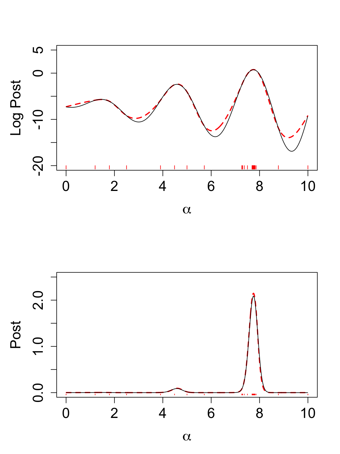
B = 100

to_plot_data <- BO_result_list[[20]]
to_plot_data$logpos <- log(to_plot_data$pos)
to_plot_data_obs <- BO_result_original_list[[20]]
y_min <- -20; y_max <- 5

mar.default <- c(5,4,4,2)
par(mar = mar.default + c(0, 1, 0, 0), mfrow = c(2, 1))
plot(to_plot_data$logpos ~ to_plot_data$x, 
       type = "l", lty = "dashed", col = "red", lwd = 2,
       ylab = "Log Post", xlab = expression(alpha),
       ylim = c(y_min, y_max), cex.lab = 1.5, cex.axis = 1.5)
lines((true_log_post(x)) ~ x, lwd = 1)
y_offset <- 0.03 * (y_max - y_min) # adjust offset as needed
for(x_val in to_plot_data_obs$x_original) {
    segments(x_val, y_min, x_val, y_min - y_offset, col = "red")
}

plot(exp(to_plot_data$logpos) ~ to_plot_data$x, 
       type = "l", lty = "dashed", col = "red", lwd = 2,
       ylab = "Post", xlab = expression(alpha), ylim = c(0, 2.5), cex.lab = 1.5, cex.axis = 1.5)
lines(exp(true_log_post(x)) ~ x, lwd = 1)
y_min <- -0.03
y_offset <- 0.01 * (2) # adjust offset as needed
for(x_val in to_plot_data_obs$x_original) {
    segments(x_val, y_min, x_val, y_min - y_offset, col = "red")
}

Past versions of unnamed-chunk-22-1.png

Version	Author	Date
ff55aef	Ziang Zhang	2025-04-21
d35a475	Ziang Zhang	2025-04-21

KL and KS:

Let’s visualize the KL and KS divergence between the true posterior and the approximated posterior from BOSS.

KL_vec <- c()
for (i in 1:length(eval_num)) {
  KL_vec[i] <- Compute_KL(x = x, logpx = true_log_post(x), logqx = log(BO_result_list[[i]]$pos))
}
mar.default <- c(5,4,4,2)
par(mar = mar.default + c(0, 1, 0, 0))
plot((KL_vec) ~ eval_num, type = "o", ylab = "KL", xlab = "eval number: B", cex.lab = 1.5, cex.axis = 1.5)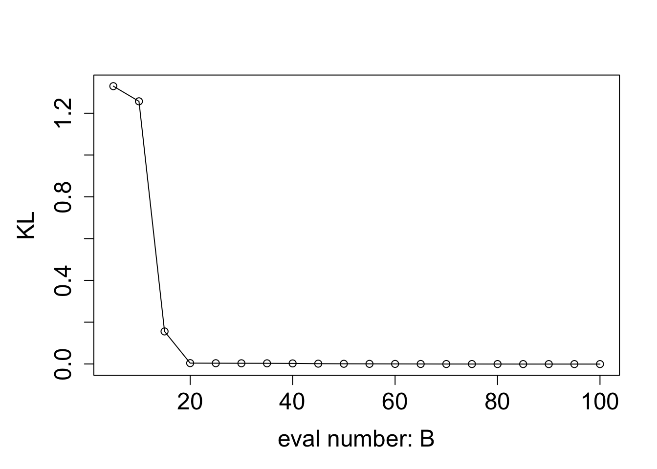

Past versions of unnamed-chunk-24-1.png

Version	Author	Date
d35a475	Ziang Zhang	2025-04-21

KS_vec <- c()
for (i in 1:length(eval_num)) {
  KS_vec[i] <- Compute_KS(x = x, px = exp(true_log_post(x)), qx = BO_result_list[[i]]$pos)
}
mar.default <- c(5,4,4,2)
par(mar = mar.default + c(0, 1, 0, 0))
plot((KS_vec) ~ eval_num, type = "o", ylab = "KS", xlab = "eval number: B", ylim = c(0,1), cex.lab = 1.5, cex.axis = 1.5)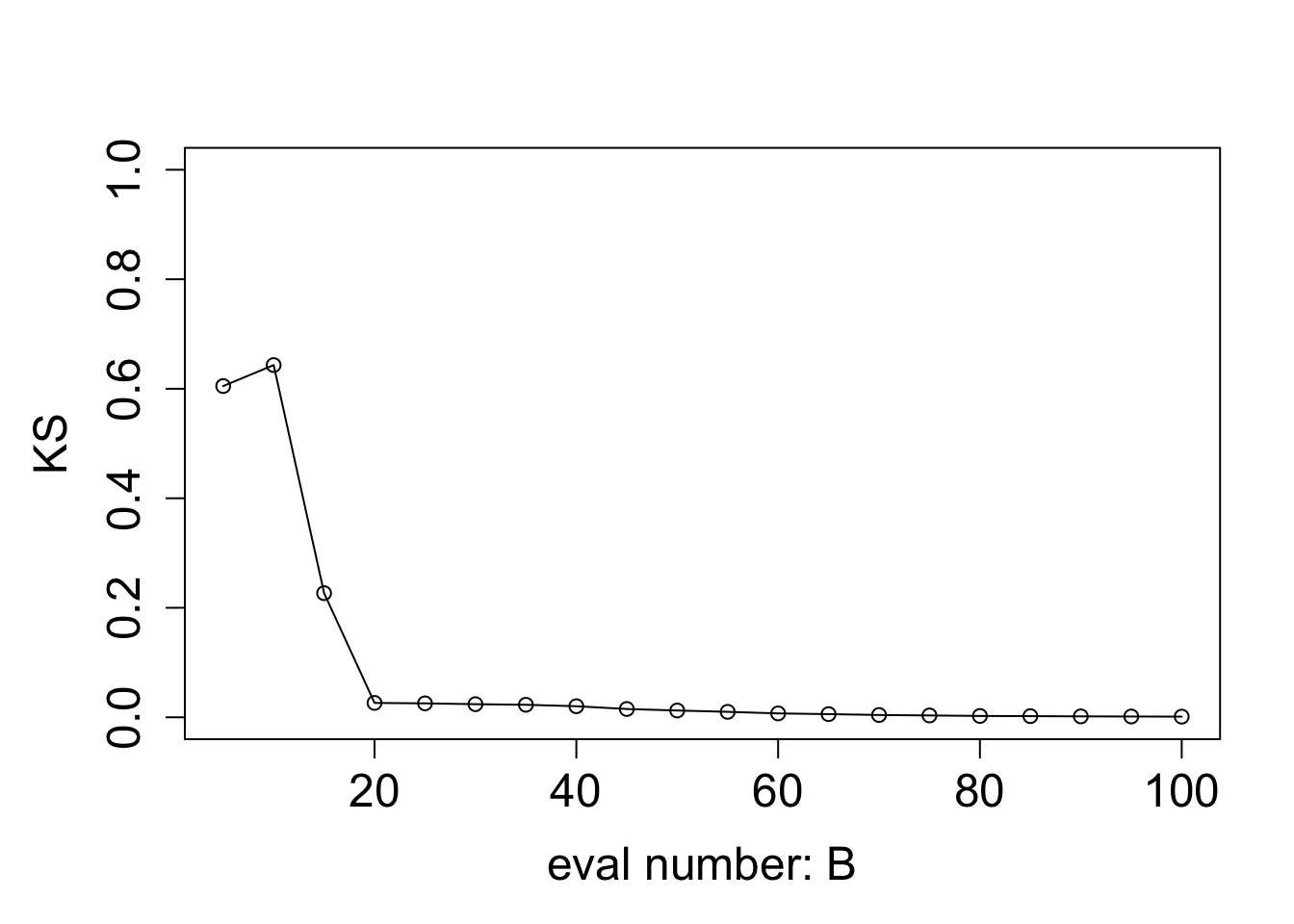

Past versions of unnamed-chunk-24-2.png

Version	Author	Date
d35a475	Ziang Zhang	2025-04-21

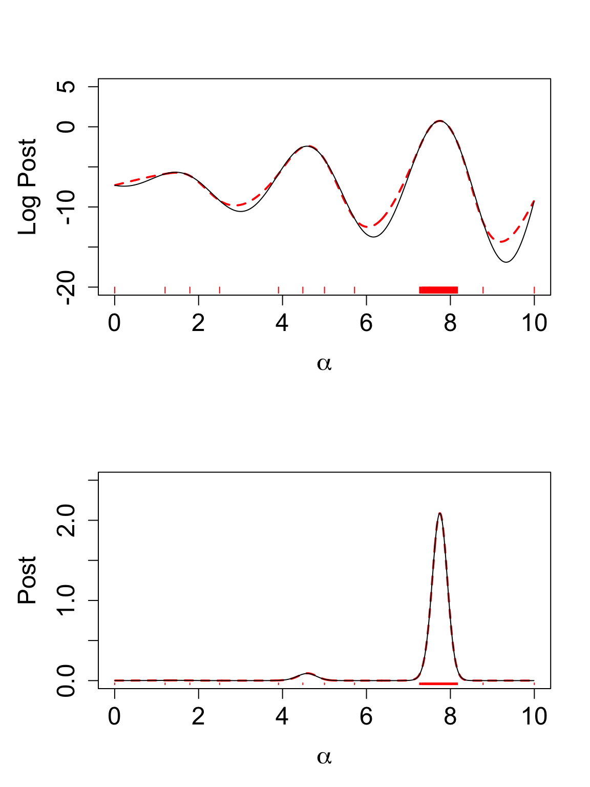
Based on the KL and KS divergence, we can the approximated posterior from BOSS is indistinguishable from the true posterior after 20 iterations of BO in the medium example.

Hard Example:

Define the log posterior function:

log_prior <- function(x){
  1
}
log_likelihood <- function(x){
  log(x + 1) * (sin(x * 4) + cos(x * 2))
}
eval_once <- function(x){
  log_prior(x) + log_likelihood(x)
}
eval_once_mapped <- function(y){
  eval_once(pnorm(y) * (upper - lower) + lower) + dnorm(y, log = T) + log(upper - lower)
}
x <- seq(0.01,9.99, by = 0.01)
y <- qnorm((x - lower)/(upper - lower))
true_log_norm_constant <- log(integrate(f = function(y) exp(eval_once_mapped(y)), lower = -Inf, upper = Inf)$value)
true_log_post_mapped <- function(y) {eval_once_mapped(y) - true_log_norm_constant}
plot((true_log_post_mapped(y)) ~ y, type = "l", cex.lab = 1.5, cex.axis = 1.5, 
     xlab = "y", ylab = "log density", lwd = 2, col = "blue")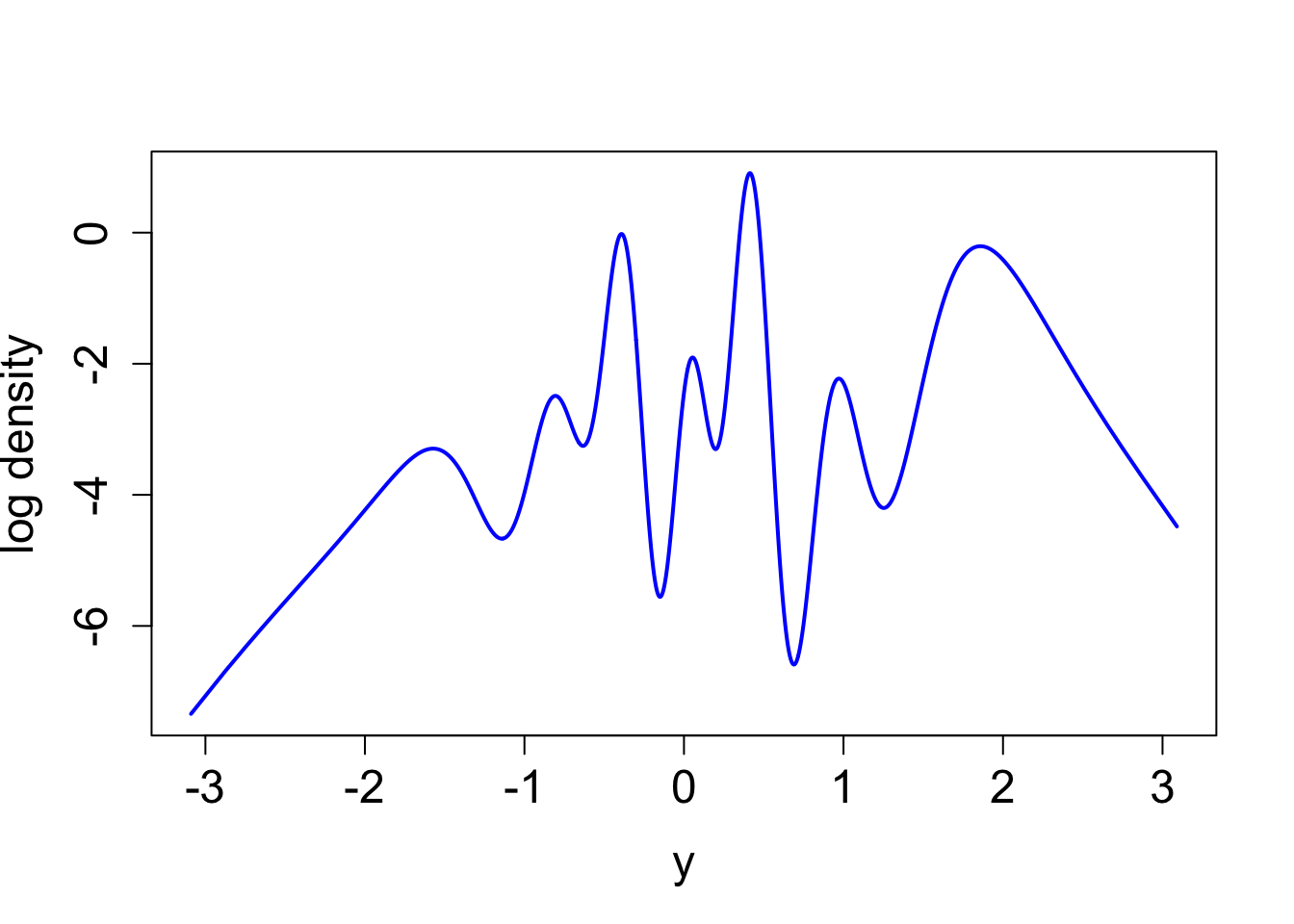

Past versions of unnamed-chunk-26-1.png

Version	Author	Date
d35a475	Ziang Zhang	2025-04-21

true_log_post <- function(x) {true_log_post_mapped(qnorm((x - lower)/(upper - lower))) - dnorm(qnorm((x - lower)/(upper - lower)), log = T) - log(upper - lower)}
integrate(function(x) exp(true_log_post(x)), lower = 0, upper = 10)

1 with absolute error < 9.1e-05

Let’s run BOSS with the above log posterior function:

objective_func <- eval_once

result_ad <- BOSS(
  func = objective_func, initial_design = 5,
  update_step = 5, max_iter = (max(eval_num) - 5),
  opt.lengthscale.grid = 100, opt.grid = 1000,
  delta = 0.01, noise_var = noise_var,
  lower = lower, upper = upper,
  AGHQ_iter_check = Inf, AGHQ_eps = 0
)
saveRDS(result_ad, file = paste0(data_path, "/result_ad_hard.rds"))

BO_result_list <- list()
BO_result_original_list <- list()
result_ad <- readRDS(file = paste0(data_path, "/result_ad_hard.rds"))
for (i in 1:length(eval_num)) {
  eval_number <- eval_num[i]

  result_ad_selected <- list(x = result_ad$result$x[1:eval_number, ],
                             x_original = result_ad$result$x_original[1:eval_number, ],
                             y = result_ad$result$y[1:eval_number])
  
  data_to_smooth <- result_ad_selected
  BO_result_original_list[[i]] <- data_to_smooth

  ff <- list()
  ff$fn <- function(y) as.numeric(surrogate(pnorm(y), data_to_smooth = data_to_smooth) + dnorm(y, log = TRUE))
  fn_vals <- sapply(y, ff$fn)

  lognormal_const <- log(integrate(f = function(y) exp(ff$fn(y)), lower = -Inf, upper = Inf)$value)
  post_y <- data.frame(y = y, pos = exp(fn_vals - lognormal_const))
  post_x <- data.frame(x = pnorm(post_y$y) * (upper - lower) + lower, post = (post_y$pos / dnorm(post_y$y))/(upper - lower) )
  
  BO_result_list[[i]] <- post_x
}
saveRDS(BO_result_list, file = paste0(data_path, "/BO_result_list_hard.rds"))
saveRDS(BO_result_original_list, file = paste0(data_path, "/BO_result_original_list_hard.rds"))

Some illustrations

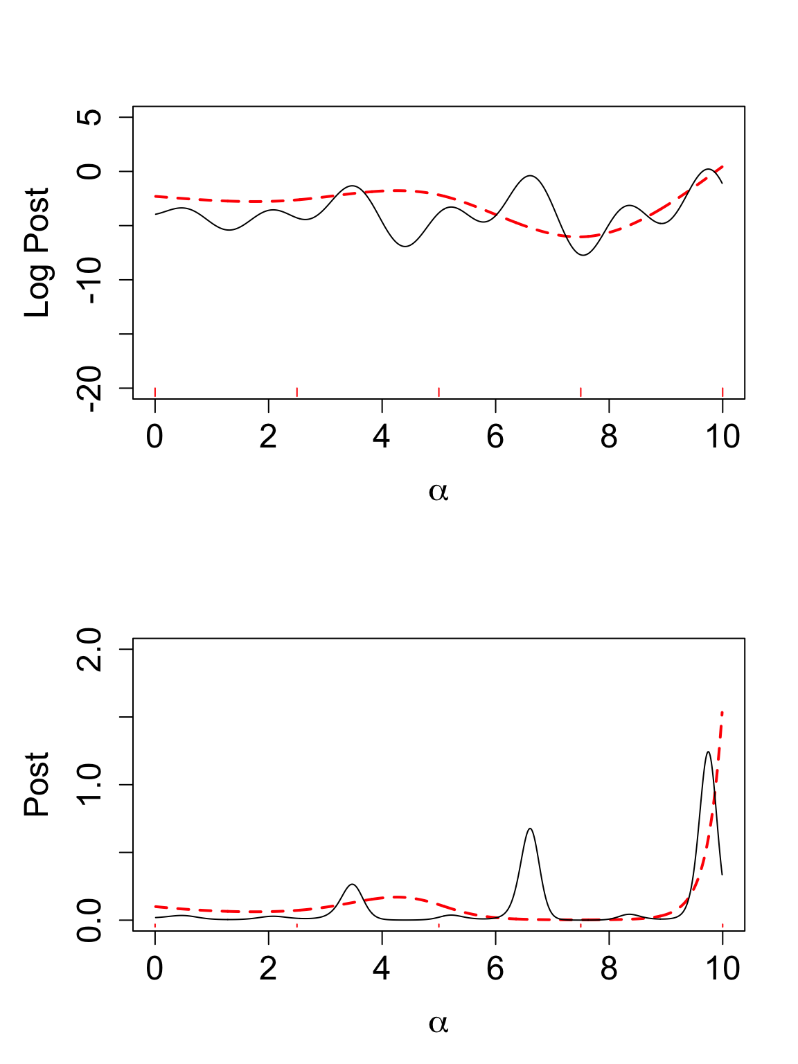
Here are some illustrations of the approximated posterior from BOSS with different numbers of BO iterations \(B\) (red: approximated posterior, black: true posterior).

BO_result_list <- readRDS(file = paste0(data_path, "/BO_result_list_hard.rds"))
BO_result_original_list <- readRDS(file = paste0(data_path, "/BO_result_original_list_hard.rds"))

B = 5

to_plot_data <- BO_result_list[[1]]
to_plot_data$logpos <- log(to_plot_data$pos)
to_plot_data_obs <- BO_result_original_list[[1]]
y_min <- -20; y_max <- 5
mar.default <- c(5,4,4,2)
par(mar = mar.default + c(0, 1, 0, 0), mfrow = c(2, 1))
plot(to_plot_data$logpos ~ to_plot_data$x, 
       type = "l", lty = "dashed", col = "red", lwd = 2,
       ylab = "Log Post", xlab = expression(alpha),
       ylim = c(y_min, y_max), cex.lab = 1.5, cex.axis = 1.5)
lines((true_log_post(x)) ~ x, lwd = 1)
y_offset <- 0.03 * (y_max - y_min) # adjust offset as needed
for(x_val in to_plot_data_obs$x_original) {
    segments(x_val, y_min, x_val, y_min - y_offset, col = "red")
}

plot(exp(to_plot_data$logpos) ~ to_plot_data$x, 
       type = "l", lty = "dashed", col = "red", lwd = 2,
       ylab = "Post", xlab = expression(alpha), ylim = c(0,2), cex.lab = 1.5, cex.axis = 1.5)
lines(exp(true_log_post(x)) ~ x, lwd = 1)
y_min <- -0.03
y_offset <- 0.01 * (2) # adjust offset as needed
for(x_val in to_plot_data_obs$x_original) {
    segments(x_val, y_min, x_val, y_min - y_offset, col = "red")
}

Past versions of unnamed-chunk-31-1.png

Version	Author	Date
ff55aef	Ziang Zhang	2025-04-21
d35a475	Ziang Zhang	2025-04-21

B = 10

to_plot_data <- BO_result_list[[2]]
to_plot_data$logpos <- log(to_plot_data$pos)
to_plot_data_obs <- BO_result_original_list[[2]]
y_min <- -20; y_max <- 5
mar.default <- c(5,4,4,2)
par(mar = mar.default + c(0, 1, 0, 0), mfrow = c(2, 1))
plot(to_plot_data$logpos ~ to_plot_data$x, 
       type = "l", lty = "dashed", col = "red", lwd = 2,
       ylab = "Log Post", xlab = expression(alpha),
       ylim = c(y_min, y_max), cex.lab = 1.5, cex.axis = 1.5)
lines((true_log_post(x)) ~ x, lwd = 1)
y_offset <- 0.03 * (y_max - y_min) # adjust offset as needed
for(x_val in to_plot_data_obs$x_original) {
    segments(x_val, y_min, x_val, y_min - y_offset, col = "red")
}

plot(exp(to_plot_data$logpos) ~ to_plot_data$x, 
       type = "l", lty = "dashed", col = "red", lwd = 2,
       ylab = "Post", xlab = expression(alpha), ylim = c(0,2), cex.lab = 1.5, cex.axis = 1.5)
lines(exp(true_log_post(x)) ~ x, lwd = 1)
y_min <- -0.03
y_offset <- 0.01 * (2) # adjust offset as needed
for(x_val in to_plot_data_obs$x_original) {
    segments(x_val, y_min, x_val, y_min - y_offset, col = "red")
}

Past versions of unnamed-chunk-32-1.png

Version	Author	Date
ff55aef	Ziang Zhang	2025-04-21
d35a475	Ziang Zhang	2025-04-21

B = 30

to_plot_data <- BO_result_list[[6]]
to_plot_data$logpos <- log(to_plot_data$pos)
to_plot_data_obs <- BO_result_original_list[[6]]
y_min <- -20; y_max <- 5
mar.default <- c(5,4,4,2)
par(mar = mar.default + c(0, 1, 0, 0), mfrow = c(2, 1))
plot(to_plot_data$logpos ~ to_plot_data$x, 
       type = "l", lty = "dashed", col = "red", lwd = 2,
       ylab = "Log Post", xlab = expression(alpha),
       ylim = c(y_min, y_max), cex.lab = 1.5, cex.axis = 1.5)
lines((true_log_post(x)) ~ x, lwd = 1)
y_offset <- 0.03 * (y_max - y_min) # adjust offset as needed
for(x_val in to_plot_data_obs$x_original) {
    segments(x_val, y_min, x_val, y_min - y_offset, col = "red")
}

plot(exp(to_plot_data$logpos) ~ to_plot_data$x, 
       type = "l", lty = "dashed", col = "red", lwd = 2,
       ylab = "Post", xlab = expression(alpha), ylim = c(0,2), cex.lab = 1.5, cex.axis = 1.5)
lines(exp(true_log_post(x)) ~ x, lwd = 1)
y_min <- -0.03
y_offset <- 0.01 * (2) # adjust offset as needed
for(x_val in to_plot_data_obs$x_original) {
    segments(x_val, y_min, x_val, y_min - y_offset, col = "red")
}

Past versions of unnamed-chunk-33-1.png

Version	Author	Date
ff55aef	Ziang Zhang	2025-04-21
d35a475	Ziang Zhang	2025-04-21

B = 100

to_plot_data <- BO_result_list[[20]]
to_plot_data$logpos <- log(to_plot_data$pos)
to_plot_data_obs <- BO_result_original_list[[20]]
y_min <- -20; y_max <- 5
mar.default <- c(5,4,4,2)
par(mar = mar.default + c(0, 1, 0, 0), mfrow = c(2, 1))
plot(to_plot_data$logpos ~ to_plot_data$x, 
       type = "l", lty = "dashed", col = "red", lwd = 2,
       ylab = "Log Post", xlab = expression(alpha),
       ylim = c(y_min, y_max), cex.lab = 1.5, cex.axis = 1.5)
lines((true_log_post(x)) ~ x, lwd = 1)
y_offset <- 0.03 * (y_max - y_min) # adjust offset as needed
for(x_val in to_plot_data_obs$x_original) {
    segments(x_val, y_min, x_val, y_min - y_offset, col = "red")
}
y_min <- -20; y_max <- 5
plot(exp(to_plot_data$logpos) ~ to_plot_data$x, 
       type = "l", lty = "dashed", col = "red", lwd = 2,
       ylab = "Post", xlab = expression(alpha), ylim = c(0,2), cex.lab = 1.5, cex.axis = 1.5)
lines(exp(true_log_post(x)) ~ x, lwd = 1)
y_min <- -0.03
y_offset <- 0.01 * (2) # adjust offset as needed
for(x_val in to_plot_data_obs$x_original) {
    segments(x_val, y_min, x_val, y_min - y_offset, col = "red")
}

Past versions of unnamed-chunk-34-1.png

Version	Author	Date
ff55aef	Ziang Zhang	2025-04-21
d35a475	Ziang Zhang	2025-04-21

Compute KL and KS:

Let’s visualize the KL and KS divergence between the true posterior and the approximated posterior from BOSS.

KL_vec <- c()
for (i in 1:length(eval_num)) {
  KL_vec[i] <- Compute_KL(x = x, logpx = true_log_post(x), logqx = log(BO_result_list[[i]]$pos))
}

mar.default <- c(5,4,4,2)
par(mar = mar.default + c(0, 1, 0, 0))
plot((KL_vec) ~ eval_num, type = "o", ylab = "KL", xlab = "eval number: B", cex.lab = 1.5, cex.axis = 1.5)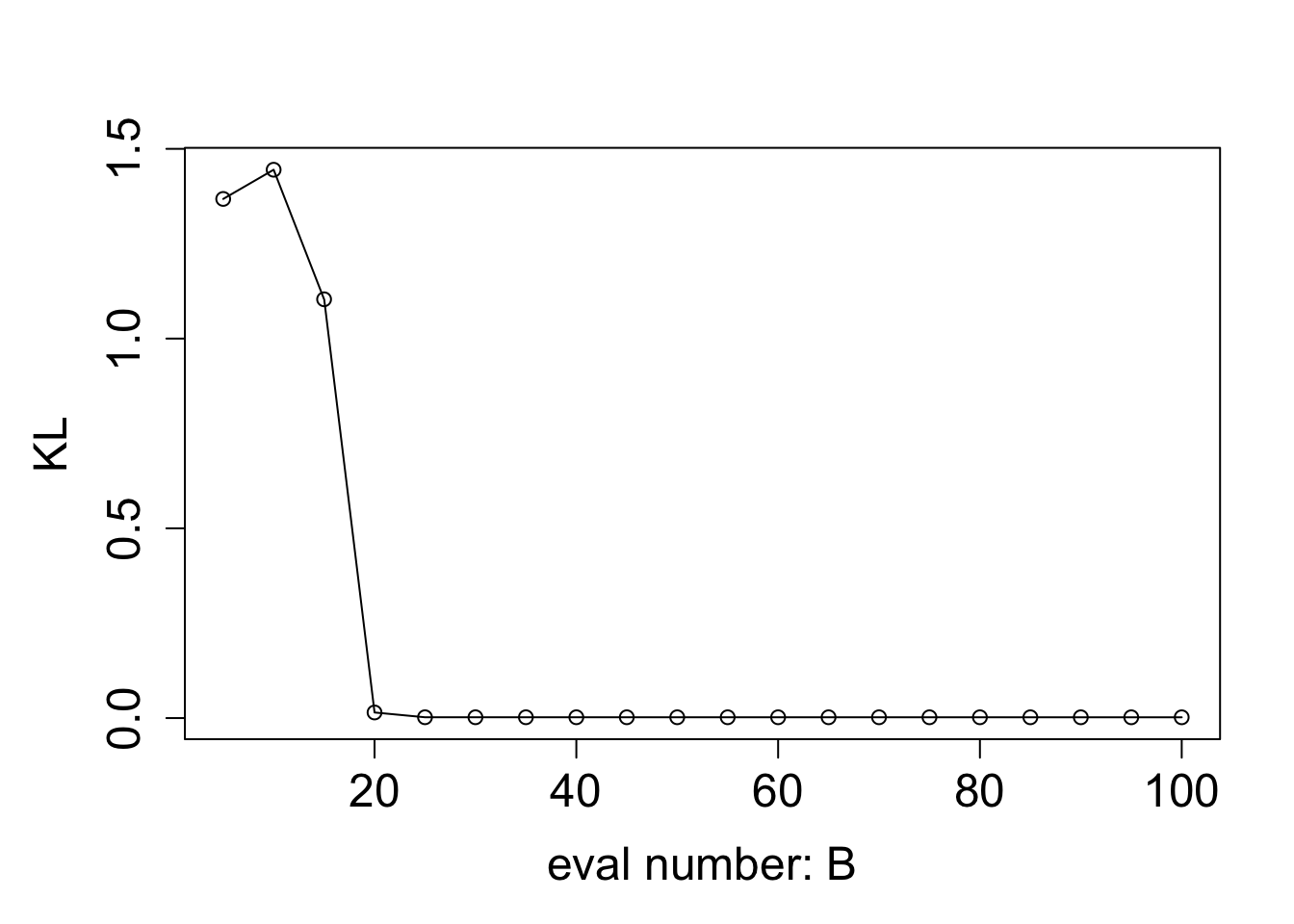

Past versions of unnamed-chunk-36-1.png

Version	Author	Date
ff55aef	Ziang Zhang	2025-04-21
d35a475	Ziang Zhang	2025-04-21

KS_vec <- c()
for (i in 1:length(eval_num)) {
  KS_vec[i] <- Compute_KS(x = x, px = exp(true_log_post(x)), qx = BO_result_list[[i]]$pos)
}
mar.default <- c(5,4,4,2)
par(mar = mar.default + c(0, 1, 0, 0))
plot((KS_vec) ~ eval_num, type = "o", ylab = "KS", xlab = "eval number: B", ylim = c(0,1), cex.lab = 1.5, cex.axis = 1.5)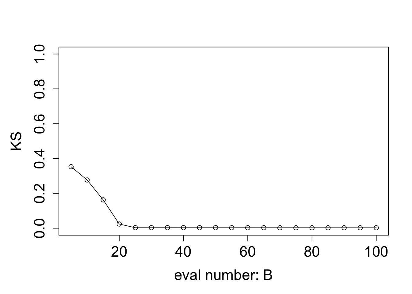

Past versions of unnamed-chunk-36-2.png

Version	Author	Date
ff55aef	Ziang Zhang	2025-04-21
d35a475	Ziang Zhang	2025-04-21

Based on the KL and KS divergence, we can the approximated posterior from BOSS is indistinguishable from the true posterior after around 20 iterations in this hard example.

Session information

sessionInfo()

R version 4.3.1 (2023-06-16)
Platform: aarch64-apple-darwin20 (64-bit)
Running under: macOS Monterey 12.7.4

Matrix products: default
BLAS:   /Library/Frameworks/R.framework/Versions/4.3-arm64/Resources/lib/libRblas.0.dylib 
LAPACK: /Library/Frameworks/R.framework/Versions/4.3-arm64/Resources/lib/libRlapack.dylib;  LAPACK version 3.11.0

locale:
[1] en_US.UTF-8/en_US.UTF-8/en_US.UTF-8/C/en_US.UTF-8/en_US.UTF-8

time zone: America/Chicago
tzcode source: internal

attached base packages:
[1] stats     graphics  grDevices utils     datasets  methods   base     

other attached packages:
[1] aghq_0.4.1      ggplot2_3.5.1   npreg_1.1.0     workflowr_1.7.1

loaded via a namespace (and not attached):
 [1] sass_0.4.9          utf8_1.2.4          generics_0.1.3     
 [4] lattice_0.22-6      stringi_1.8.4       digest_0.6.37      
 [7] magrittr_2.0.3      evaluate_1.0.1      grid_4.3.1         
[10] fastmap_1.2.0       rprojroot_2.0.4     jsonlite_1.8.9     
[13] Matrix_1.6-4        processx_3.8.4      whisker_0.4.1      
[16] ps_1.8.0            promises_1.3.0      httr_1.4.7         
[19] fansi_1.0.6         scales_1.3.0        numDeriv_2016.8-1.1
[22] jquerylib_0.1.4     cli_3.6.3           rlang_1.1.4        
[25] munsell_0.5.1       withr_3.0.2         cachem_1.1.0       
[28] yaml_2.3.10         tools_4.3.1         dplyr_1.1.4        
[31] colorspace_2.1-1    httpuv_1.6.15       vctrs_0.6.5        
[34] R6_2.5.1            lifecycle_1.0.4     git2r_0.33.0       
[37] stringr_1.5.1       fs_1.6.4            pkgconfig_2.0.3    
[40] callr_3.7.6         pillar_1.9.0        bslib_0.8.0        
[43] later_1.3.2         gtable_0.3.6        data.table_1.16.2  
[46] glue_1.8.0          Rcpp_1.0.13-1       statmod_1.5.0      
[49] mvQuad_1.0-8        highr_0.11          xfun_0.48          
[52] tibble_3.2.1        tidyselect_1.2.1    rstudioapi_0.16.0  
[55] knitr_1.48          htmltools_0.5.8.1   rmarkdown_2.28     
[58] compiler_4.3.1      getPass_0.2-4