Last updated: 2025-04-30

Checks: 7 0

Knit directory: BOSS_website/

This reproducible R Markdown analysis was created with workflowr (version 1.7.1). The Checks tab describes the reproducibility checks that were applied when the results were created. The Past versions tab lists the development history.

R Markdown file: up-to-date

Great! Since the R Markdown file has been committed to the Git repository, you know the exact version of the code that produced these results.

Environment: empty

Great job! The global environment was empty. Objects defined in the global environment can affect the analysis in your R Markdown file in unknown ways. For reproduciblity it’s best to always run the code in an empty environment.

Seed: set.seed(20250415)

The command set.seed(20250415) was run prior to running the code in the R Markdown file. Setting a seed ensures that any results that rely on randomness, e.g. subsampling or permutations, are reproducible.

Session information: recorded

Great job! Recording the operating system, R version, and package versions is critical for reproducibility.

Cache: none

Nice! There were no cached chunks for this analysis, so you can be confident that you successfully produced the results during this run.

File paths: relative

Great job! Using relative paths to the files within your workflowr project makes it easier to run your code on other machines.

Repository version: 2caf2b9

Great! You are using Git for version control. Tracking code development and connecting the code version to the results is critical for reproducibility.

The results in this page were generated with repository version 2caf2b9. See the Past versions tab to see a history of the changes made to the R Markdown and HTML files.

Note that you need to be careful to ensure that all relevant files for the analysis have been committed to Git prior to generating the results (you can use wflow_publish or wflow_git_commit). workflowr only checks the R Markdown file, but you know if there are other scripts or data files that it depends on. Below is the status of the Git repository when the results were generated:


Ignored files:
    Ignored:    .DS_Store
    Ignored:    .Rhistory
    Ignored:    .Rproj.user/
    Ignored:    analysis/.DS_Store
    Ignored:    analysis/.Rhistory
    Ignored:    code/.DS_Store
    Ignored:    data/.DS_Store
    Ignored:    data/sim1/
    Ignored:    output/.DS_Store
    Ignored:    output/sim2/.DS_Store

Untracked files:
    Untracked:  code/mortality_BG_grid.R
    Untracked:  code/mortality_NL_grid.R
    Untracked:  data/co2/
    Untracked:  data/mortality/
    Untracked:  data/simA1/
    Untracked:  output/co2/
    Untracked:  output/mortality/BOSS_result.rds
    Untracked:  output/mortality/BO_result_BG.rda
    Untracked:  output/mortality/BO_result_NL.rda
    Untracked:  output/mortality/mod_BG.rda
    Untracked:  output/mortality/mod_NL.rda
    Untracked:  output/sim1/figures/
    Untracked:  output/sim1/result_ad.rda
    Untracked:  output/sim2/BOSS_result.rda
    Untracked:  output/sim2/quad_sparse_list.rda
    Untracked:  output/simA1/

Unstaged changes:
    Modified:   analysis/problem_with_opt.rmd
    Modified:   analysis/sim1.Rmd
    Modified:   code/00_BOSS.R
    Modified:   output/mortality/result_ad_BG.rda
    Modified:   output/mortality/result_ad_NL.rda
    Modified:   output/sim1/BO_result_list.rda
    Modified:   output/sim1/BO_result_original_list.rda
    Modified:   output/sim1/all_result.rda
    Modified:   output/sim1/kl_compare.pdf
    Modified:   output/sim1/ks_compare.pdf
    Modified:   output/sim2/BO_data_to_smooth.rda
    Modified:   output/sim2/BO_result_list.rda
    Modified:   output/sim2/rel_runtime.rda

Note that any generated files, e.g. HTML, png, CSS, etc., are not included in this status report because it is ok for generated content to have uncommitted changes.

These are the previous versions of the repository in which changes were made to the R Markdown (analysis/mortality.Rmd) and HTML (docs/mortality.html) files. If you’ve configured a remote Git repository (see ?wflow_git_remote), click on the hyperlinks in the table below to view the files as they were in that past version.

File	Version	Author	Date	Message
Rmd	2caf2b9	Ziang Zhang	2025-04-30	workflowr::wflow_publish("analysis/mortality.Rmd")
html	4d0397c	Ziang Zhang	2025-04-28	Build site.
Rmd	c06fbda	Ziang Zhang	2025-04-28	workflowr::wflow_publish("analysis/mortality.Rmd")
Rmd	325128f	Ziang Zhang	2025-04-22	Update BOSS function
html	26e3b3b	Ziang Zhang	2025-04-21	Build site.
Rmd	874c7ae	Ziang Zhang	2025-04-21	workflowr::wflow_publish("analysis/mortality.Rmd")

Introduction

In this example, we consider the analysis of the weekly all-cause mortality counts in the Netherlands and Bulgaria. The all-cause mortality data is obtained from the , which contains the country-level weekly death counts from 2015 to 2022.

To make inference of the change-point, we consider the following model for the weekly-mortality: \[\begin{equation} \begin{aligned} y(t_i)|\mu(t_i) &\overset{ind}{\sim} \text{Poisson}(\mu(t_i)), \\ \log(\mu(t_i)) &= \begin{cases} g_{tr,\text{pre}}(t_i) + g_{s,\text{pre}}(t_i) & \text{if } t_i \leq a, \\ g_{tr,\text{pos}}(t_i) + g_{s,\text{pos}}(t_i) & \text{if } t_i > a. \end{cases}\\ g_{tr,\text{pre}}(t_i) \sim &\text{IWP}_2(\sigma_{tr,\text{pre}}), \ g_{tr,\text{pos}}(t_i) \sim \text{IWP}_2(\sigma_{tr,\text{pos}}), \\ g_{s,\text{pre}}(t_i) \sim &\text{sGP}(\sigma_{s,\text{pre}}), \ g_{s,\text{pos}}(t_i) \sim \text{sGP}(\sigma_{s,\text{pos}}). \end{aligned} \end{equation}\]

Here $Y(t_i)$ denotes the observed weekly mortality at time $t_i$, where the unit of $t_i$ is converted to year; the conditioning parameter $\alpha$ denotes the change-point of the mortality dynamic, and is assigned an uniform prior between the first week of the year 2019 and the first week of the year 2022. We decompose the dynamic of mortality rate into the smooth long-term trend ($g_{tr,\text{pre}}$ or $g_{tr,\text{pos}}$) and the seasonal component ($g_{s,\text{pre}}$ or $g_{s,\text{pos}}$) with yearly variation. The trends are modeled using independent second order Integrated Wiener processes ($\text{IWP}_2$) and the seasonal components are modeled using independent seasonal Gaussian processes ($) $ with yearly periodicity and four harmonic terms. The boundary conditions of IWP or sGP are fixed such that neither the mortality rate $\mu$ nor its derivative will have a discontinuity at the change point $\alpha$. For priors on the variance parameters, we put independent exponential priors on their corresponding five-year predictive standard deviations, with prior median $0.01$ for $g_{tr,\text{pre}}$ and $g_{s,\text{pre}}$, and median $1$ for $g_{tr,\text{pos}}$ and $g_{s,\text{pos}}$.

West Europe: Neitherlands

Data

library(tidyverse)

── Attaching core tidyverse packages ──────────────────────── tidyverse 2.0.0 ──
✔ dplyr     1.1.4     ✔ readr     2.1.5
✔ forcats   1.0.0     ✔ stringr   1.5.1
✔ ggplot2   3.5.1     ✔ tibble    3.2.1
✔ lubridate 1.9.3     ✔ tidyr     1.3.1
✔ purrr     1.0.2     
── Conflicts ────────────────────────────────────────── tidyverse_conflicts() ──
✖ dplyr::filter() masks stats::filter()
✖ dplyr::lag()    masks stats::lag()
ℹ Use the conflicted package (<http://conflicted.r-lib.org/>) to force all conflicts to become errors

library(BayesGP)
library(npreg)

Package 'npreg' version 1.1.0
Type 'citation("npreg")' to cite this package.

set.seed(123)
noise_var = 1e-6
function_path <- "./code"
output_path <- "./output/mortality"
data_path <- "./data/mortality"
source(paste0(function_path, "/00_BOSS.R"))

cFile <- paste0(data_path, "/world_mortality.csv")
world_death = read.table(cFile, header = TRUE, sep = ",", stringsAsFactors = FALSE)

### West EU: NL
NL_death <- world_death %>% filter(country_name == "Netherlands")
NL_death$date <- make_date(year = NL_death$year) + weeks(NL_death$time)
NL_death$x <- as.numeric(NL_death$date)/365.25; 
ref_val <- min(NL_death$x)
NL_death$x <- NL_death$x - ref_val
plot(NL_death$deaths ~ NL_death$date)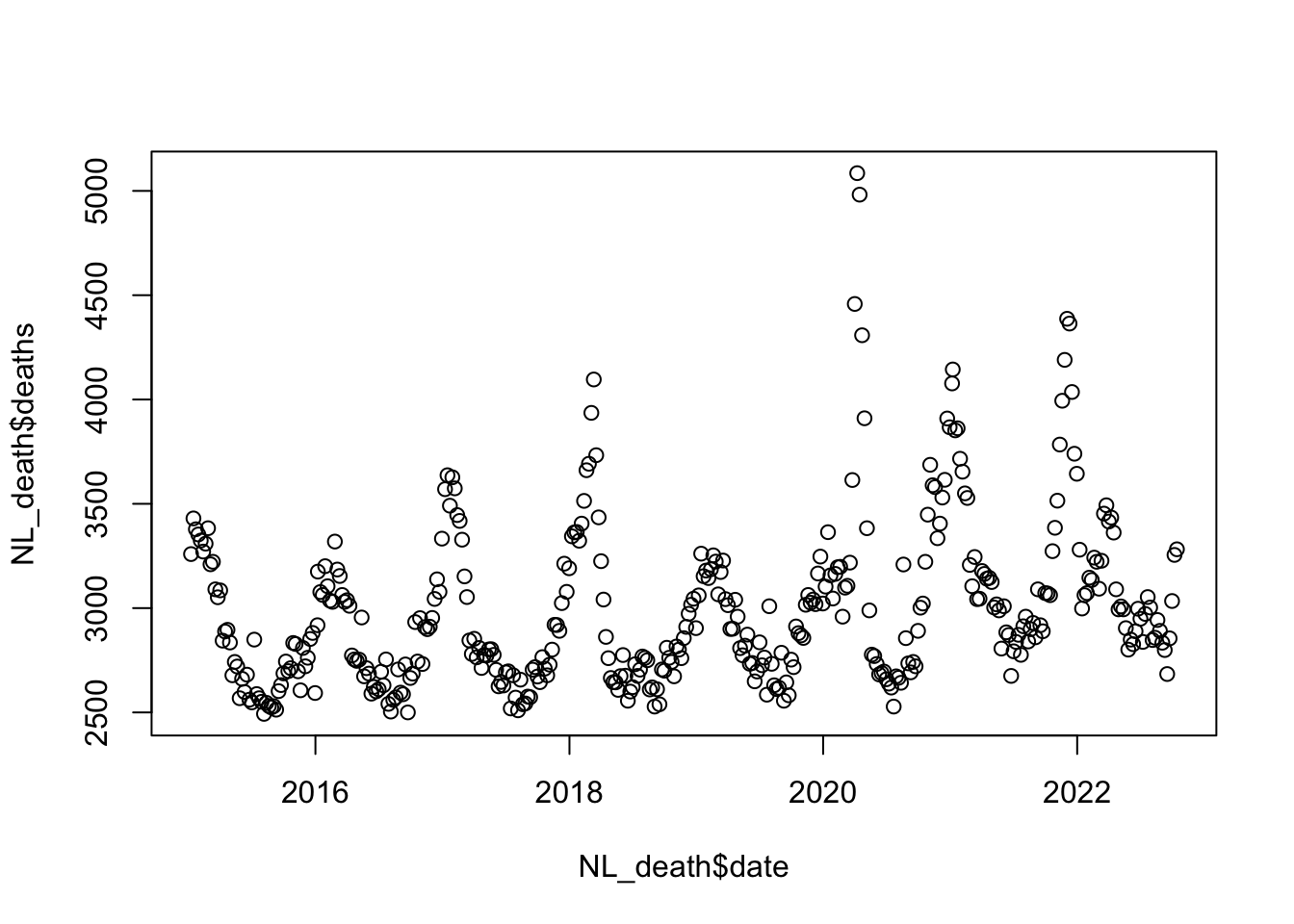

Version	Author	Date
26e3b3b	Ziang Zhang	2025-04-21

BOSS

fit_once <- function(alpha, data){
  a_fit <- alpha
  data$x1 <- ifelse(data$x <= a_fit, (a_fit - data$x), 0); 
  data$x2 <- ifelse(data$x > a_fit, (data$x - a_fit), 0);
  data$xx1 <- data$x1
  data$xx2 <- data$x2
  
  data$cov1 <- cos(2*pi*data$x)
  data$cov2 <- sin(2*pi*data$x)
  
  data$cov3 <- cos(4*pi*data$x)
  data$cov4 <- sin(4*pi*data$x)
  
  data$cov5 <- cos(8*pi*data$x)
  data$cov6 <- sin(8*pi*data$x)
  
  data$cov7 <- cos(16*pi*data$x)
  data$cov8 <- sin(16*pi*data$x)
  
  data$index <- 1:nrow(data)
  
  mod <- model_fit(formula = deaths ~ cov1 + cov2 + cov3 + cov4 + cov5 + cov6 + cov7 + cov8 +
                     f(x1, model = "sGP", period = 1, sd.prior = list(param = list(u = 0.01, alpha = 0.5), h = 5), boundary.prior = list(prec = c(Inf, Inf, Inf, Inf, Inf, Inf, Inf, Inf)), k = 20, region = c(0,8), m = 4) +
                     f(x2, model = "sGP", period = 1, sd.prior = list(param = list(u = 1, alpha = 0.5), h = 5), boundary.prior = list(prec = c(Inf, Inf, Inf, Inf, Inf, Inf, Inf, Inf)), k = 20, region = c(0,8), m = 4) +
                     f(xx1, model = "IWP", order = 2, initial_location = "min",
                       sd.prior = list(param = 0.01, h = 5), k = 20, boundary.prior = list(prec = c(Inf))) +
                     f(xx2, model = "IWP", order = 2, initial_location = "min",
                       sd.prior = list(param = 1, h = 5), k = 20, boundary.prior = list(prec = c(Inf))),
                   data = data, method = "aghq", family = "Poisson", aghq_k = 4
  )
  mod
}

eval_once <- function(alpha, data = NL_death){
  mod <- fit_once(alpha = alpha, data = data)
  (mod$mod$normalized_posterior$lognormconst)
} 

surrogate <- function(xvalue, data_to_smooth){
  data_to_smooth$y <- data_to_smooth$y - mean(data_to_smooth$y)
  predict(ss(x = as.numeric(data_to_smooth$x), y = data_to_smooth$y, df = length(unique(as.numeric(data_to_smooth$x))), m = 2, all.knots = TRUE), x = xvalue)$y
}

lower = 0.5; upper = 7.2
objective_func <- eval_once

eval_number <- 100; optim.n = 50
result_ad <- BOSS(eval_once,
  update_step = 5, max_iter = eval_number, delta = 0.01,
  lower = lower, upper = upper, 
  noise_var = noise_var,
  interpolation = "ss",
  initial_design = 5, optim.n = optim.n,
  # modal_iter_check = 1,  modal_check_warmup = 20, modal_k.nn = 5, modal_eps = 0, criterion = "modal",
  criterion = "KL", KL.grid = 3000, KL_check_warmup = 5, KL_iter_check = 5, KL_eps = 0
)
save(result_ad, file = paste0(output_path, "/result_ad_NL.rda"))

data_to_smooth <- result_ad$result
data_to_smooth$x <- as.numeric(result_ad$result$x)[order(as.numeric(result_ad$result$x))]
data_to_smooth$x_original <- as.numeric(result_ad$result$x_original)[order(as.numeric(result_ad$result$x))]
data_to_smooth$y <- as.numeric(result_ad$result$y)[order(as.numeric(result_ad$result$x))]
data_to_smooth$y <- data_to_smooth$y - max(data_to_smooth$y)

ff <- list()
ff$fn <- function(y){
    as.numeric(
    surrogate(
      y,
      data_to_smooth = data_to_smooth
    )
  )
}

x_vals <- (seq(
  from = lower,
  to = upper,
  length.out = 1000
) - lower) / (upper - lower)
fn_vals <- sapply(x_vals, ff$fn)
post_x <- data.frame(x = x_vals, fx = exp(fn_vals))

dx <- diff(x_vals)
integral_approx <- sum(0.5 * (post_x$fx[-1] + post_x$fx[-length(post_x$fx)]) * dx)
post_x$pos <- post_x$fx / integral_approx


BO_result_NL <- data.frame(x = (lower + x_vals * (upper - lower)),
                        pos = post_x$pos / (upper - lower))
BO_result_NL$year <- as.Date((BO_result_NL$x + ref_val)*365.25)
save(BO_result_NL, file = paste0(output_path, "/BO_result_NL.rda"))

Take a look at the diagnostic plot:

load(paste0(output_path, "/result_ad_NL.rda"))
plot(result_ad$KL_result$KL ~ result_ad$KL_result$i, type = 'o', ylab = "KL", xlab = "Iteration")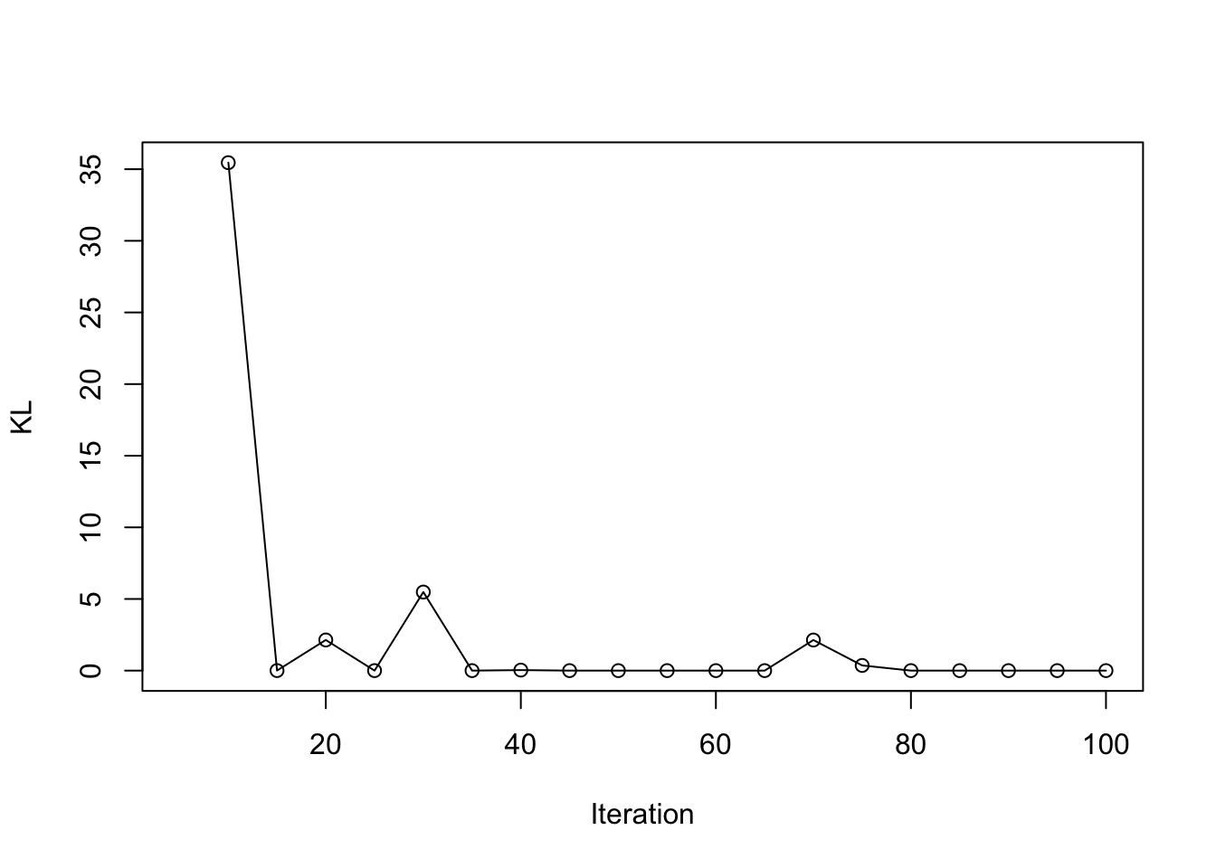

Version	Author	Date
4d0397c	Ziang Zhang	2025-04-28
26e3b3b	Ziang Zhang	2025-04-21

load(paste0(output_path, "/BO_result_NL.rda"))
ggplot() +
    geom_line(data = BO_result_NL, aes(x = year, y = pos), color = "red", size = 1) +
    xlab("") +
    ylab("Density") +
    scale_x_date(
      limits = as.Date(c("2019-12-01", "2021-01-01")),
      date_labels = "%b %y", 
      date_breaks = "3 month"
    ) +
    theme_minimal() +
    theme(text = element_text(size = 15), axis.text = element_text(size = 15))

Warning: Using `size` aesthetic for lines was deprecated in ggplot2 3.4.0.
ℹ Please use `linewidth` instead.
This warning is displayed once every 8 hours.
Call `lifecycle::last_lifecycle_warnings()` to see where this warning was
generated.

Warning: Removed 838 rows containing missing values or values outside the scale range
(`geom_line()`).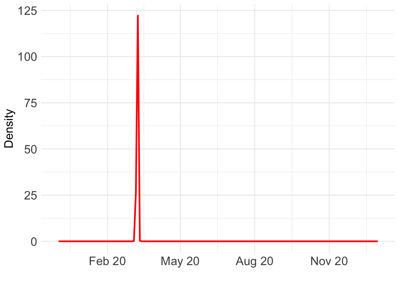

Which day is most likely?

as.Date((BO_result_NL$x[which.max(BO_result_NL$pos)] + ref_val)*365.25)

[1] "2020-03-09"

Take a look at the fit:

my_alpha_NL <- (BO_result_NL$x[which.max(BO_result_NL$pos)])

mod_NL <- fit_once(alpha = my_alpha_NL, data = NL_death)
save(mod_NL, file = paste0(output_path, "/mod_NL.rda"))

load(paste0(output_path, "/mod_NL.rda"))
f1 <- predict(mod_NL, variable = "x1", only.samples = T, boundary.condition = "no", newdata = mod_NL$instances[[1]]@data, include.intercept = F)
f1$x <- my_alpha_NL - f1$x
f2 <- predict(mod_NL, variable = "x2", only.samples = T, boundary.condition = "no", newdata = mod_NL$instances[[1]]@data, include.intercept = F)
f2$x <- f2$x + my_alpha_NL
f1 <- distinct(f1, x, .keep_all = TRUE); f2 <- distinct(f2, x, .keep_all = TRUE)
f <- rbind(f1, f2) %>% arrange(x); f <- distinct(f, x, .keep_all = TRUE)
g1 <- predict(mod_NL, variable = "xx1", only.samples = T, boundary.condition = "no", newdata = mod_NL$instances[[1]]@data, include.intercept = F)
g1$x <- my_alpha_NL - g1$x
g2 <- predict(mod_NL, variable = "xx2", only.samples = T, boundary.condition = "no", newdata = mod_NL$instances[[1]]@data, include.intercept = F)
g2$x <- g2$x + my_alpha_NL
g1 <- distinct(g1, x, .keep_all = TRUE); g2 <- distinct(g2, x, .keep_all = TRUE)
g <- rbind(g1, g2) %>% arrange(x); g <- distinct(g, x, .keep_all = TRUE)

fixed_pred <- cbind(cos(2*pi*f$x), sin(2*pi*f$x), cos(4*pi*f$x), sin(4*pi*f$x), cos(8*pi*f$x), sin(8*pi*f$x), cos(16*pi*f$x), sin(16*pi*f$x), 1) %*% t(sample_fixed_effect(mod_NL, variables = c("cov1", "cov2", "cov3", "cov4", "cov5", "cov6", "cov7", "cov8", "intercept")))
f_all <- f[,-1] + fixed_pred + g[,-1]
f_summ <- data.frame(mean = apply(f_all, 1, mean), upper = apply(f_all, 1, quantile, 0.975), upper = apply(f_all, 1, quantile, 0.025))

par(cex.axis = 1.5,   # Increase font size of axis text
    cex.lab = 1.5,    # Increase font size of axis labels
    cex.main = 1.6)   # Increase font size of main titles
matplot(y = exp(f_summ), x = as.Date((f$x+ ref_val)*365.25), type = "l", col = c("black","red", "red"), lty = c("solid", "dashed", "dashed"),
        ylab = "Weekly Deaths", xlab = "")
abline(v = as.Date((my_alpha_NL+ ref_val)*365.25), lty = "dashed", col = "purple")
points(NL_death$deaths ~ as.Date((NL_death$x+ ref_val)*365.25), cex = 0.2, col = "black")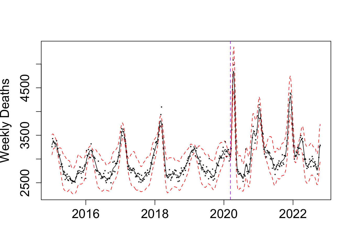

Exact grid

As the oracle method, we implement the exact grid approach with a equally spaced grid of 1000 points.

n_cores <- 5
res_list  <- mclapply(x_vals, eval_once, mc.cores = n_cores)
exact_vals <- unlist(res_list)
exact_grid_result_NL <- data.frame(x = x_vals, exact_vals = exact_vals)
save(exact_grid_result_NL, file = paste0(output_path, "/exact_grid_result_NL_unnormalized.rda"))

How much difference between the optimal alpha found by BOSS and the exact grid?

load(paste0(output_path, "/exact_grid_result_NL_unnormalized.rda"))

The relative difference is 0.

Take a look at the posterior distribution of the exact grid:

exact_grid_result_NL$exact_vals <- exact_grid_result_NL$exact_vals - max(exact_grid_result_NL$exact_vals)
exact_grid_result_NL$fx <- exp(exact_grid_result_NL$exact_vals)
# Calculate the differences between adjacent x values
dx <- diff(exact_grid_result_NL$x)
# Compute the trapezoidal areas and sum them up
integral_approx <- sum(0.5 * (exact_grid_result_NL$fx[-1] + exact_grid_result_NL$fx[-length(exact_grid_result_NL$fx)]) * dx)
exact_grid_result_NL$pos <- exact_grid_result_NL$fx / integral_approx
exact_grid_result_NL$pos <- exact_grid_result_NL$pos
# convert to time
exact_grid_result_NL$year <- as.Date((exact_grid_result_NL$x + ref_val)*365.25)

load(paste0(output_path, "/BO_result_NL.rda"))

# Select needed columns and add Method labels
BO_result_NL_sub <- BO_result_NL %>%
  select(year, pos) %>%
  mutate(Method = "BOSS")

exact_grid_result_NL_sub <- exact_grid_result_NL %>%
  select(year, pos) %>%
  mutate(Method = "Exact Grid")

# Combine
plot_data <- bind_rows(BO_result_NL_sub, exact_grid_result_NL_sub)

# Now plot
ggplot(plot_data, aes(x = year, y = pos, color = Method, linetype = Method)) +
  geom_line(size = 0.6) +
  xlab("") +
  ylab("Density") +
  scale_x_date(
    limits = as.Date(c("2019-12-01", "2021-01-01")),
    date_labels = "%b %y", 
    date_breaks = "3 month"
  ) +
  theme_minimal() +
  theme(
    text = element_text(size = 15), 
    axis.text = element_text(size = 15),
    legend.position = c(0.8, 0.8),
    legend.title = element_blank(),
    legend.text = element_text(size = 15)
  ) +
  scale_color_manual(values = c("BOSS" = "blue", "Exact Grid" = "red")) +
  scale_linetype_manual(values = c("BOSS" = "solid", "Exact Grid" = "dashed"))

Warning: A numeric `legend.position` argument in `theme()` was deprecated in ggplot2
3.5.0.
ℹ Please use the `legend.position.inside` argument of `theme()` instead.
This warning is displayed once every 8 hours.
Call `lifecycle::last_lifecycle_warnings()` to see where this warning was
generated.

Warning: Removed 1676 rows containing missing values or values outside the scale range
(`geom_line()`).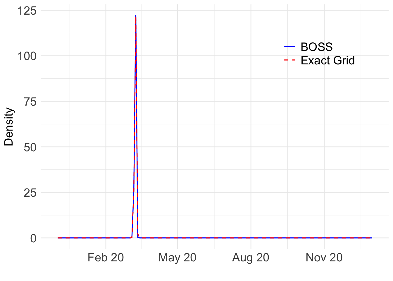

Version	Author	Date
4d0397c	Ziang Zhang	2025-04-28
26e3b3b	Ziang Zhang	2025-04-21

The BOSS surrogate posterior distribution is shown in blue, while the exact grid posterior distribution is shown in red. The BOSS surrogate in this case is indistinguishable from the posterior distribution obtained from the exact grid, but only takes a fraction of the time to compute.

East Europe: Bulgaria

Data

BG_death <- world_death %>% filter(country_name == "Bulgaria")
BG_death$date <- make_date(year = BG_death$year) + weeks(BG_death$time)
BG_death$x <- as.numeric(BG_death$date)/365.25; 
ref_val <- min(BG_death$x)
BG_death$x <- BG_death$x - ref_val
plot(BG_death$deaths ~ BG_death$date)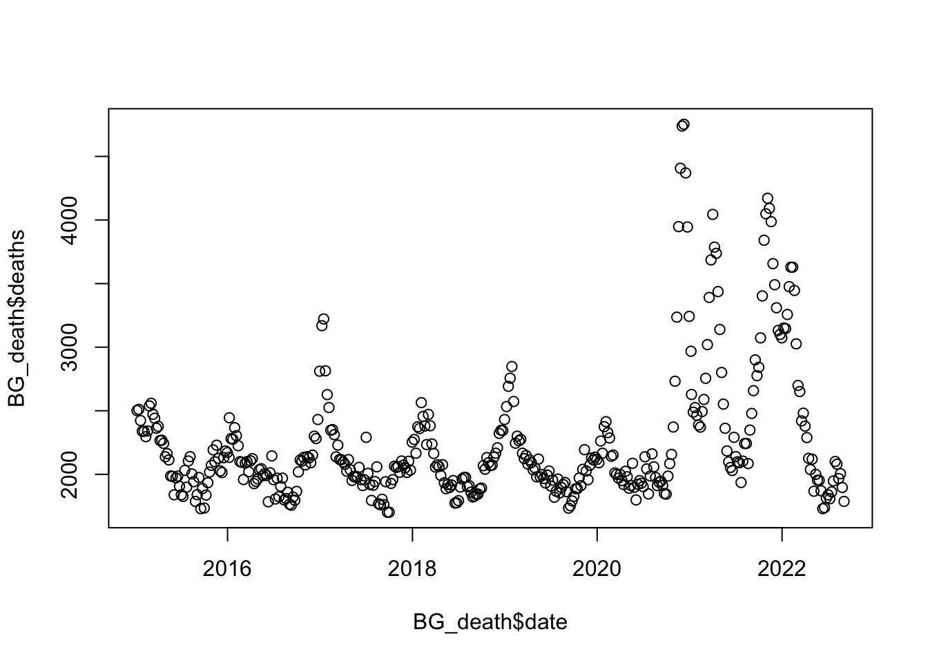

BOSS

eval_once <- function(alpha, data = BG_death){
  mod <- fit_once(alpha = alpha, data = data)
  (mod$mod$normalized_posterior$lognormconst)
} 
objective_func <- eval_once

result_ad <- BOSS(eval_once,
  update_step = 5, max_iter = eval_number, delta = 0.01,
  lower = lower, upper = upper, 
  noise_var = noise_var,
  initial_design = 5, optim.n = optim.n,
  # modal_iter_check = 1,  modal_check_warmup = 20, modal_k.nn = 5, modal_eps = 0, criterion = "modal",
  interpolation = "ss",
  criterion = "KL", KL.grid = 3000, KL_check_warmup = 5, KL_iter_check = 5, KL_eps = 0
)
save(result_ad, file = paste0(output_path, "/result_ad_BG.rda"))

data_to_smooth <- result_ad$result
data_to_smooth$x <- as.numeric(result_ad$result$x)[order(as.numeric(result_ad$result$x))]
data_to_smooth$x_original <- as.numeric(result_ad$result$x_original)[order(as.numeric(result_ad$result$x))]
data_to_smooth$y <- as.numeric(result_ad$result$y)[order(as.numeric(result_ad$result$x))]
data_to_smooth$y <- data_to_smooth$y - max(data_to_smooth$y)

ff <- list()
ff$fn <- function(y){
    as.numeric(
    surrogate(
      y,
      data_to_smooth = data_to_smooth
    )
  )
}


x_vals <- (seq(
  from = lower,
  to = upper,
  length.out = 1000
) - lower) / (upper - lower)
fn_vals <- sapply(x_vals, ff$fn)
post_x <- data.frame(x = x_vals, fx = exp(fn_vals))

dx <- diff(x_vals)
integral_approx <- sum(0.5 * (post_x$fx[-1] + post_x$fx[-length(post_x$fx)]) * dx)
post_x$pos <- post_x$fx / integral_approx

BO_result_BG <- data.frame(x = (lower + x_vals * (upper - lower)),
                        pos = post_x$pos / (upper - lower))
BO_result_BG$year <- as.Date((BO_result_BG$x + ref_val)*365.25)
save(BO_result_BG, file = paste0(output_path, "/BO_result_BG.rda"))

Take a look at the diagnostic plot:

load(paste0(output_path, "/result_ad_BG.rda"))
plot(result_ad$KL_result$KL ~ result_ad$KL_result$i, type = 'o', ylab = "KL", xlab = "Iteration")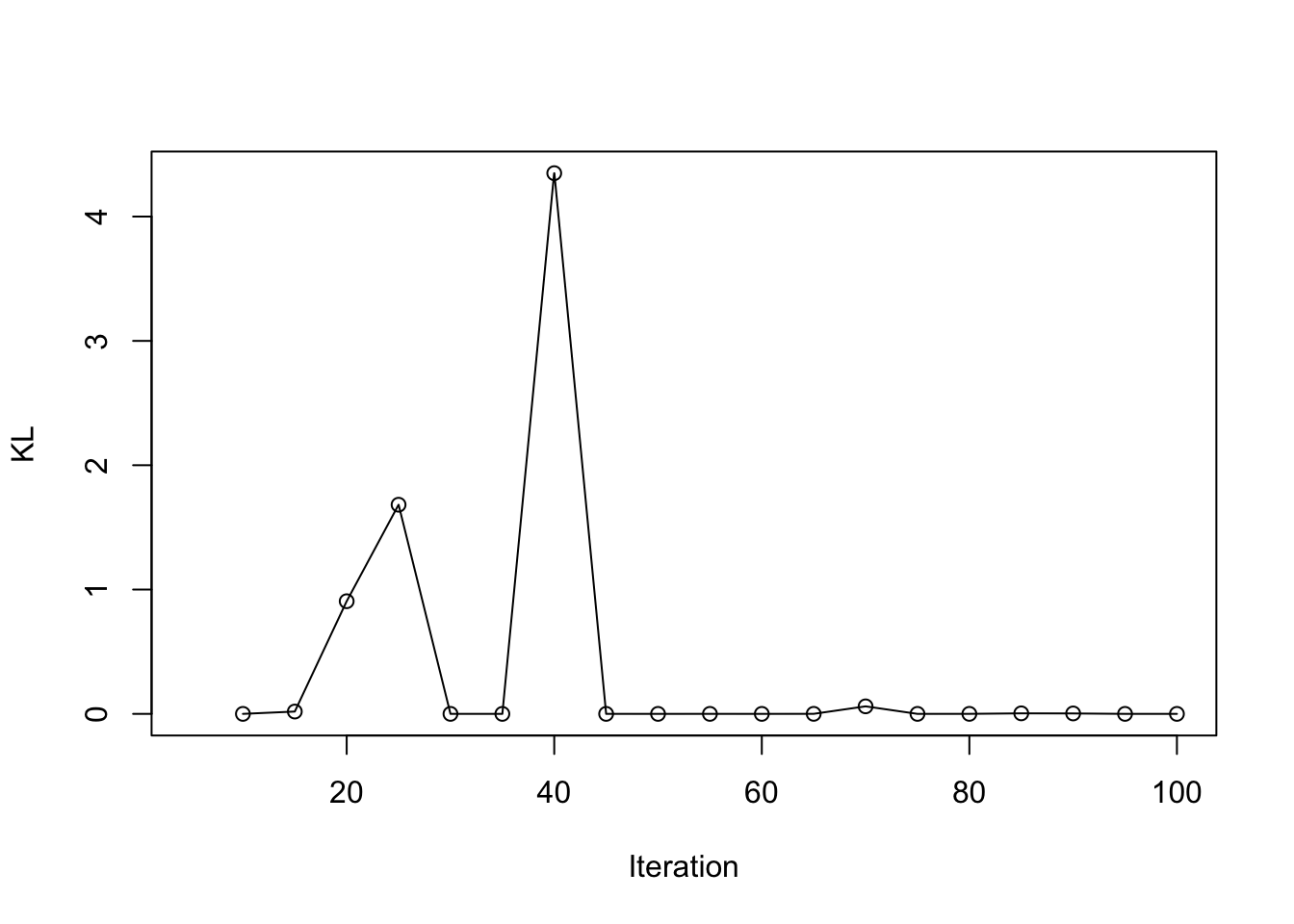

Version	Author	Date
4d0397c	Ziang Zhang	2025-04-28
26e3b3b	Ziang Zhang	2025-04-21

load(paste0(output_path, "/BO_result_BG.rda"))
ggplot() +
    geom_line(data = BO_result_BG, aes(x = year, y = pos), color = "red", size = 1) +
    xlab("") +
    ylab("Density") +
    scale_x_date(
      limits = as.Date(c("2019-12-01", "2021-01-01")),
      date_labels = "%b %y", 
      date_breaks = "3 month"
    ) +
    theme_minimal() +
    theme(text = element_text(size = 15), axis.text = element_text(size = 15))

Warning: Removed 838 rows containing missing values or values outside the scale range
(`geom_line()`).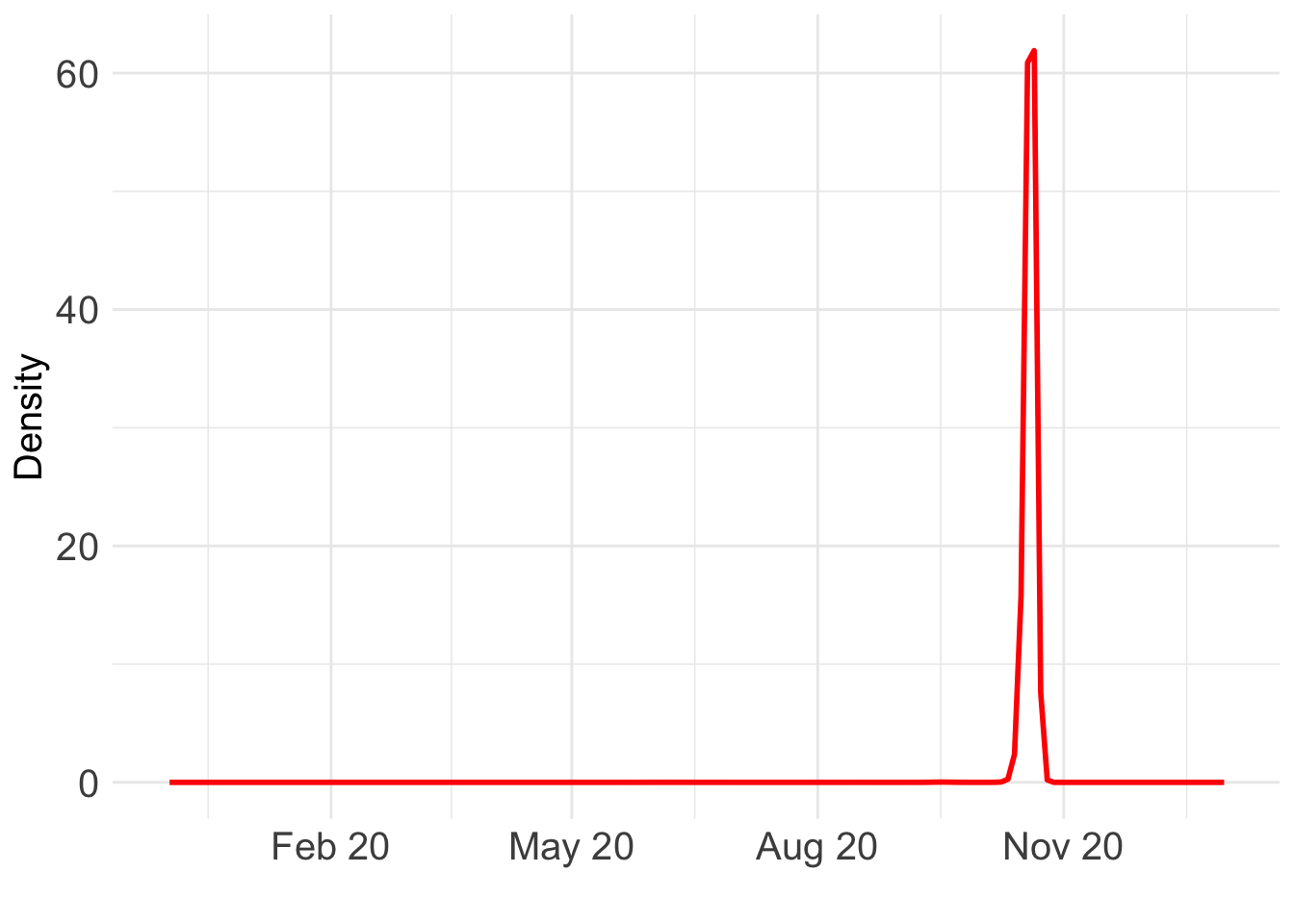

Which day is most likely?

as.Date((BO_result_BG$x[which.max(BO_result_BG$pos)] + ref_val)*365.25)

[1] "2020-10-20"

Take a look at the fit:

my_alpha_BG <- (BO_result_BG$x[which.max(BO_result_BG$pos)])

mod_BG <- fit_once(alpha = my_alpha_BG, data = BG_death)
save(mod_BG, file = paste0(output_path, "/mod_BG.rda"))

load(paste0(output_path, "/mod_BG.rda"))
f1 <- predict(mod_BG, variable = "x1", only.samples = T, boundary.condition = "no", newdata = mod_BG$instances[[1]]@data, include.intercept = F)
f1$x <- my_alpha_BG - f1$x
f2 <- predict(mod_BG, variable = "x2", only.samples = T, boundary.condition = "no", newdata = mod_BG$instances[[1]]@data, include.intercept = F)
f2$x <- f2$x + my_alpha_BG
f1 <- distinct(f1, x, .keep_all = TRUE); f2 <- distinct(f2, x, .keep_all = TRUE)
f <- rbind(f1, f2) %>% arrange(x); f <- distinct(f, x, .keep_all = TRUE)
g1 <- predict(mod_BG, variable = "xx1", only.samples = T, boundary.condition = "no", newdata = mod_BG$instances[[1]]@data, include.intercept = F)
g1$x <- my_alpha_BG - g1$x
g2 <- predict(mod_BG, variable = "xx2", only.samples = T, boundary.condition = "no", newdata = mod_BG$instances[[1]]@data, include.intercept = F)
g2$x <- g2$x + my_alpha_BG
g1 <- distinct(g1, x, .keep_all = TRUE); g2 <- distinct(g2, x, .keep_all = TRUE)
g <- rbind(g1, g2) %>% arrange(x); g <- distinct(g, x, .keep_all = TRUE)

fixed_pred <- cbind(cos(2*pi*f$x), sin(2*pi*f$x), cos(4*pi*f$x), sin(4*pi*f$x), cos(8*pi*f$x), sin(8*pi*f$x), cos(16*pi*f$x), sin(16*pi*f$x), 1) %*% t(sample_fixed_effect(mod_BG, variables = c("cov1", "cov2", "cov3", "cov4", "cov5", "cov6", "cov7", "cov8", "intercept")))
f_all <- f[,-1] + fixed_pred + g[,-1]
f_summ <- data.frame(mean = apply(f_all, 1, mean), upper = apply(f_all, 1, quantile, 0.975), upper = apply(f_all, 1, quantile, 0.025))

par(cex.axis = 1.5,   # Increase font size of axis text
    cex.lab = 1.5,    # Increase font size of axis labels
    cex.main = 1.6)   # Increase font size of main titles
matplot(y = exp(f_summ), x = as.Date((f$x+ ref_val)*365.25), type = "l", col = c("black","red", "red"), lty = c("solid", "dashed", "dashed"),
        ylab = "Weekly Deaths", xlab = "")
abline(v = as.Date((my_alpha_BG+ ref_val)*365.25), lty = "dashed", col = "purple")
points(BG_death$deaths ~ as.Date((BG_death$x+ ref_val)*365.25), cex = 0.2, col = "black")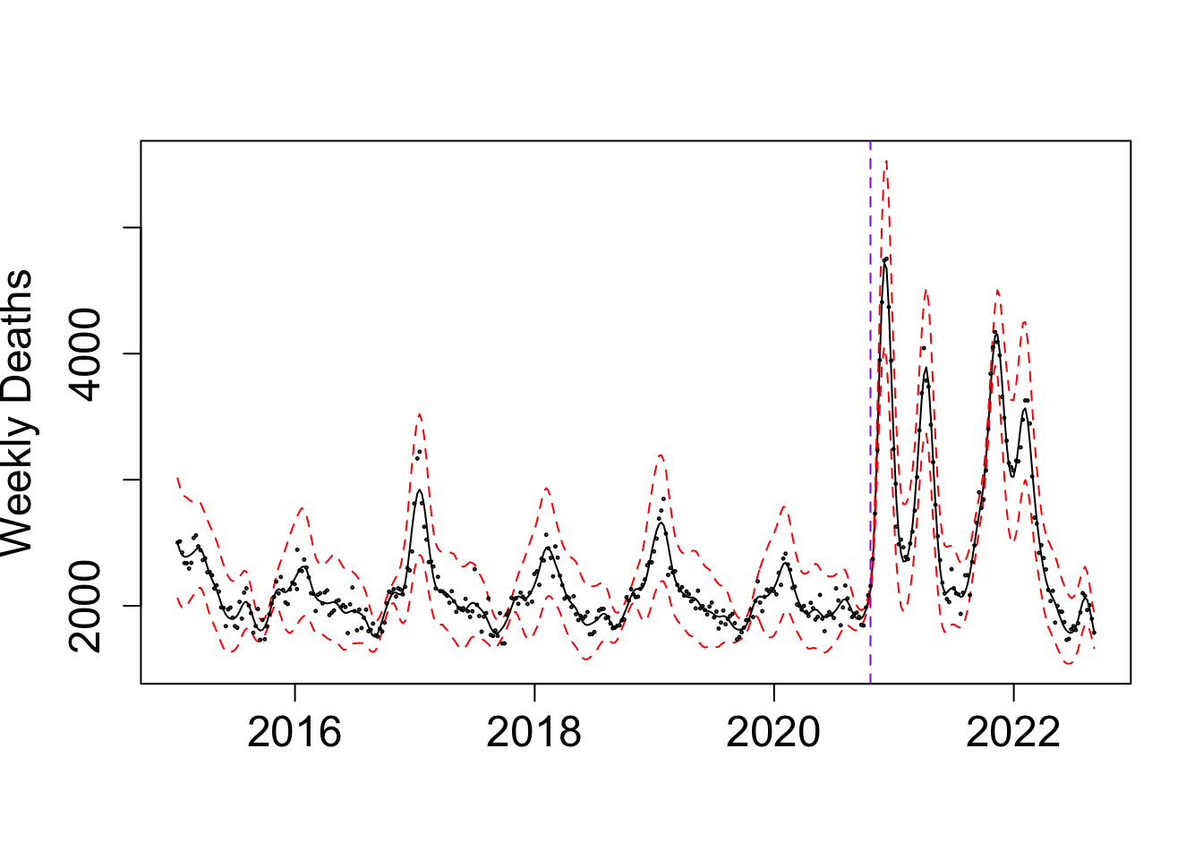

Exact grid

As the oracle method, we implement the exact grid approach with a equally spaced grid of 1000 points.

n_cores <- 5
res_list  <- mclapply(x_vals, eval_once, mc.cores = n_cores)
exact_vals <- unlist(res_list)
exact_grid_result_BG <- data.frame(x = x_vals, exact_vals = exact_vals)
save(exact_grid_result_BG, file = paste0(output_path, "/exact_grid_result_BG_unnormalized.rda"))

How much difference between the optimal alpha found by BOSS and the exact grid?

load(paste0(output_path, "/exact_grid_result_BG_unnormalized.rda"))

The relative difference is 0.

Take a look at the posterior distribution of the exact grid:

exact_grid_result_BG$exact_vals <- exact_grid_result_BG$exact_vals - max(exact_grid_result_BG$exact_vals)
exact_grid_result_BG$fx <- exp(exact_grid_result_BG$exact_vals)
# Calculate the differences between adjacent x values
dx <- diff(exact_grid_result_BG$x)
# Compute the trapezoidal areas and sum them up
integral_approx <- sum(0.5 * (exact_grid_result_BG$fx[-1] + exact_grid_result_BG$fx[-length(exact_grid_result_BG$fx)]) * dx)
exact_grid_result_BG$pos <- exact_grid_result_BG$fx / integral_approx
exact_grid_result_BG$pos <- exact_grid_result_BG$pos
# convert to time
exact_grid_result_BG$year <- as.Date((exact_grid_result_BG$x + ref_val)*365.25)

load(paste0(output_path, "/BO_result_BG.rda"))

# Select needed columns and add Method labels
BO_result_BG_sub <- BO_result_BG %>%
  select(year, pos) %>%
  mutate(Method = "BOSS")

exact_grid_result_BG_sub <- exact_grid_result_BG %>%
  select(year, pos) %>%
  mutate(Method = "Exact Grid")

# Combine
plot_data <- bind_rows(BO_result_BG_sub, exact_grid_result_BG_sub)

# Now plot
ggplot(plot_data, aes(x = year, y = pos, color = Method, linetype = Method)) +
  geom_line(size = 0.6) +
  xlab("") +
  ylab("Density") +
  scale_x_date(
    limits = as.Date(c("2019-12-01", "2021-01-01")),
    date_labels = "%b %y", 
    date_breaks = "3 month"
  ) +
  theme_minimal() +
  theme(
    text = element_text(size = 15), 
    axis.text = element_text(size = 15),
    legend.position = c(0.2, 0.8),
    legend.title = element_blank(),
    legend.text = element_text(size = 15)
  ) +
  scale_color_manual(values = c("BOSS" = "blue", "Exact Grid" = "red")) +
  scale_linetype_manual(values = c("BOSS" = "solid", "Exact Grid" = "dashed"))

Warning: Removed 1676 rows containing missing values or values outside the scale range
(`geom_line()`).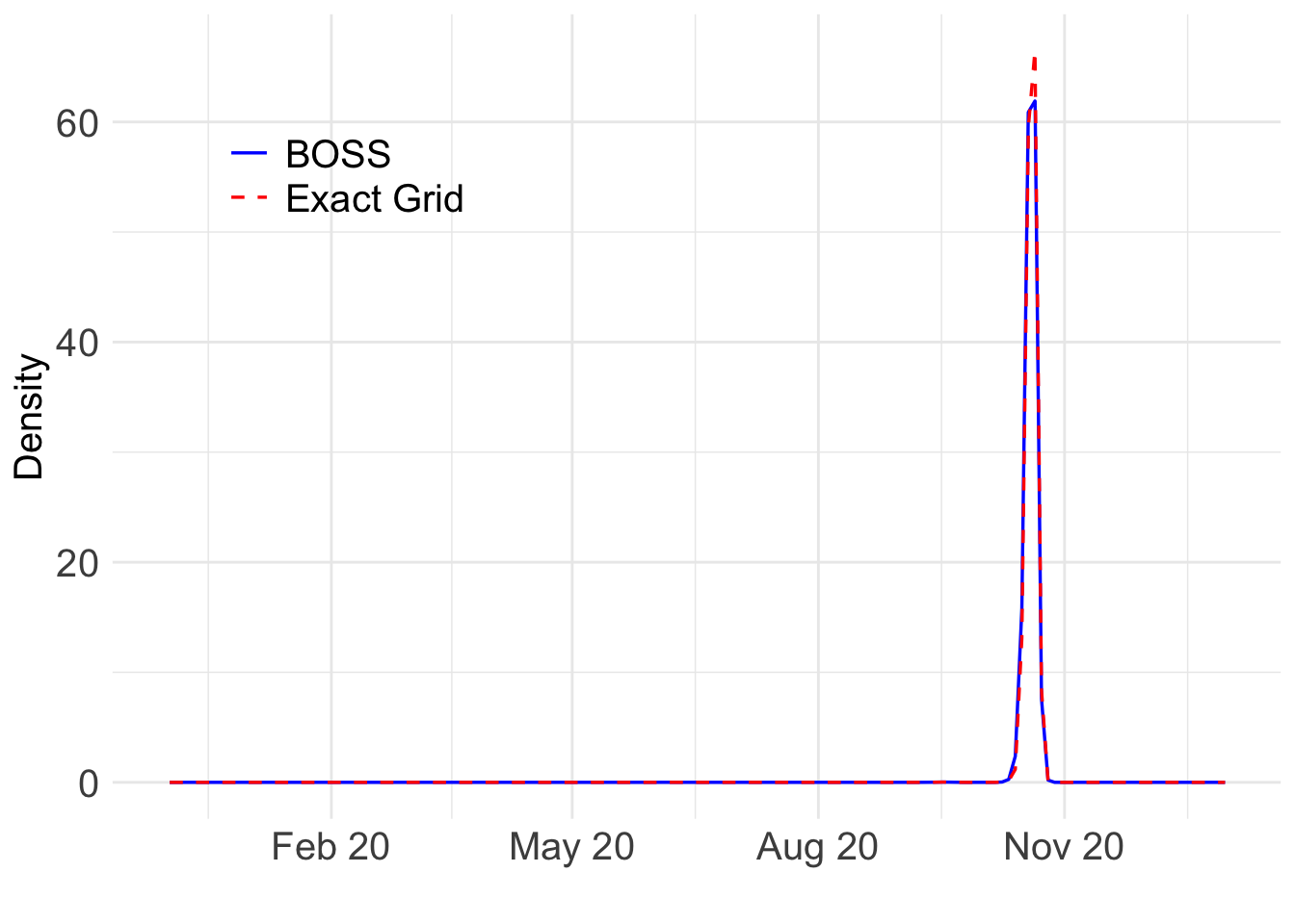

sessionInfo()

R version 4.3.1 (2023-06-16)
Platform: aarch64-apple-darwin20 (64-bit)
Running under: macOS Monterey 12.7.4

Matrix products: default
BLAS:   /Library/Frameworks/R.framework/Versions/4.3-arm64/Resources/lib/libRblas.0.dylib 
LAPACK: /Library/Frameworks/R.framework/Versions/4.3-arm64/Resources/lib/libRlapack.dylib;  LAPACK version 3.11.0

locale:
[1] en_US.UTF-8/en_US.UTF-8/en_US.UTF-8/C/en_US.UTF-8/en_US.UTF-8

time zone: America/Toronto
tzcode source: internal

attached base packages:
[1] stats     graphics  grDevices utils     datasets  methods   base     

other attached packages:
 [1] npreg_1.1.0     BayesGP_0.1.3   lubridate_1.9.3 forcats_1.0.0  
 [5] stringr_1.5.1   dplyr_1.1.4     purrr_1.0.2     readr_2.1.5    
 [9] tidyr_1.3.1     tibble_3.2.1    ggplot2_3.5.1   tidyverse_2.0.0
[13] workflowr_1.7.1

loaded via a namespace (and not attached):
 [1] gtable_0.3.6       TMB_1.9.15         xfun_0.48          bslib_0.8.0       
 [5] ks_1.14.3          processx_3.8.4     lattice_0.22-6     callr_3.7.6       
 [9] tzdb_0.4.0         bitops_1.0-9       vctrs_0.6.5        tools_4.3.1       
[13] ps_1.8.0           generics_0.1.3     aghq_0.4.1         fansi_1.0.6       
[17] cluster_2.1.6      highr_0.11         fds_1.8            pkgconfig_2.0.3   
[21] KernSmooth_2.23-24 Matrix_1.6-4       data.table_1.16.2  lifecycle_1.0.4   
[25] compiler_4.3.1     farver_2.1.2       git2r_0.33.0       statmod_1.5.0     
[29] munsell_0.5.1      getPass_0.2-4      mvQuad_1.0-8       httpuv_1.6.15     
[33] rainbow_3.8        htmltools_0.5.8.1  sass_0.4.9         RCurl_1.98-1.16   
[37] yaml_2.3.10        pracma_2.4.4       later_1.3.2        pillar_1.9.0      
[41] crayon_1.5.3       jquerylib_0.1.4    whisker_0.4.1      MASS_7.3-60       
[45] cachem_1.1.0       mclust_6.1.1       tidyselect_1.2.1   digest_0.6.37     
[49] mvtnorm_1.3-1      stringi_1.8.4      splines_4.3.1      labeling_0.4.3    
[53] pcaPP_2.0-5        rprojroot_2.0.4    fastmap_1.2.0      grid_4.3.1        
[57] colorspace_2.1-1   cli_3.6.3          magrittr_2.0.3     utf8_1.2.4        
[61] withr_3.0.2        scales_1.3.0       promises_1.3.0     timechange_0.3.0  
[65] rmarkdown_2.28     httr_1.4.7         deSolve_1.40       hms_1.1.3         
[69] evaluate_1.0.1     knitr_1.48         rlang_1.1.4        Rcpp_1.0.13-1     
[73] hdrcde_3.4         fda_6.2.0          glue_1.8.0         rstudioapi_0.16.0 
[77] jsonlite_1.8.9     R6_2.5.1           fs_1.6.4

Example 2: Change Points in All-Cause Mortality

Ziang Zhang

2025-04-18

Introduction

West Europe: Neitherlands

Data

BOSS

Exact grid

East Europe: Bulgaria

Data

BOSS

Exact grid