Convergence Diagnostic
Ziang Zhang
2025-04-22
Last updated: 2025-04-22
Checks: 7 0
Knit directory: BOSS_website/
This reproducible R Markdown analysis was created with workflowr (version 1.7.1). The Checks tab describes the reproducibility checks that were applied when the results were created. The Past versions tab lists the development history.
Great! Since the R Markdown file has been committed to the Git repository, you know the exact version of the code that produced these results.
Great job! The global environment was empty. Objects defined in the global environment can affect the analysis in your R Markdown file in unknown ways. For reproduciblity it’s best to always run the code in an empty environment.
The command set.seed(20250415) was run prior to running
the code in the R Markdown file. Setting a seed ensures that any results
that rely on randomness, e.g. subsampling or permutations, are
reproducible.
Great job! Recording the operating system, R version, and package versions is critical for reproducibility.
Nice! There were no cached chunks for this analysis, so you can be confident that you successfully produced the results during this run.
Great job! Using relative paths to the files within your workflowr project makes it easier to run your code on other machines.
Great! You are using Git for version control. Tracking code development and connecting the code version to the results is critical for reproducibility.
The results in this page were generated with repository version 6af839c. See the Past versions tab to see a history of the changes made to the R Markdown and HTML files.
Note that you need to be careful to ensure that all relevant files for
the analysis have been committed to Git prior to generating the results
(you can use wflow_publish or
wflow_git_commit). workflowr only checks the R Markdown
file, but you know if there are other scripts or data files that it
depends on. Below is the status of the Git repository when the results
were generated:
Ignored files:
    Ignored:    .DS_Store
    Ignored:    .Rhistory
    Ignored:    .Rproj.user/
    Ignored:    analysis/.DS_Store
    Ignored:    analysis/.Rhistory
    Ignored:    code/.DS_Store
    Ignored:    data/.DS_Store
    Ignored:    data/sim1/
    Ignored:    output/.DS_Store
    Ignored:    output/sim2/.DS_Store

Untracked files:
    Untracked:  code/mortality_BG_grid.R
    Untracked:  code/mortality_NL_grid.R
    Untracked:  data/co2/
    Untracked:  data/mortality/
    Untracked:  data/simA1/
    Untracked:  output/co2/
    Untracked:  output/mortality/
    Untracked:  output/sim2/quad_sparse_list.rda
    Untracked:  output/simA1/

Unstaged changes:
    Modified:   output/sim2/BO_data_to_smooth.rda
    Modified:   output/sim2/BO_result_list.rda
    Modified:   output/sim2/rel_runtime.rda
Note that any generated files, e.g. HTML, png, CSS, etc., are not included in this status report because it is ok for generated content to have uncommitted changes.
These are the previous versions of the repository in which changes were
made to the R Markdown (analysis/diagnostic.rmd) and HTML
(docs/diagnostic.html) files. If you’ve configured a remote
Git repository (see ?wflow_git_remote), click on the
hyperlinks in the table below to view the files as they were in that
past version.
| File | Version | Author | Date | Message |
|---|---|---|---|---|
| Rmd | 6af839c | Ziang Zhang | 2025-04-22 | workflowr::wflow_publish("analysis/diagnostic.rmd") |
| html | b02f19c | david.li | 2025-04-22 | Build site. |
| Rmd | 8b99f87 | david.li | 2025-04-22 | wflow_publish("analysis/diagnostic.Rmd") |
| html | b5d1ce2 | Ziang Zhang | 2025-04-22 | Build site. |
| Rmd | 074cea3 | Ziang Zhang | 2025-04-22 | workflowr::wflow_publish("analysis/diagnostic.rmd") |
| html | 6bb1cbf | Ziang Zhang | 2025-04-22 | Build site. |
| Rmd | 8550bd7 | Ziang Zhang | 2025-04-22 | workflowr::wflow_publish("analysis/diagnostic.rmd") |
Introduction
In this tutorial, we examine several diagnostic tools that can be used to assess the convergence of BOSS.
For now, let’s assume the following true (log) posterior:
library(npreg)Package 'npreg' version 1.1.0
Type 'citation("npreg")' to cite this package.library(ggplot2)
library(aghq)
set.seed(123)
noise_var = 1e-6
function_path <- "./code"
output_path <- "./output/simA1"
data_path <- "./data/simA1"
source(paste0(function_path, "/00_BOSS.R"))
lower = 0; upper = 10
log_prior <- function(x){
1
}
log_likelihood <- function(x){
log(x + 1) * (sin(x * 4) + cos(x * 2))
}
eval_once <- function(x){
log_prior(x) + log_likelihood(x)
}
eval_once_mapped <- function(y){
eval_once(pnorm(y) * (upper - lower) + lower) + dnorm(y, log = T) + log(upper - lower)
}
x <- seq(0.01,9.99, by = 0.01)
y <- qnorm((x - lower)/(upper - lower))
true_log_norm_constant <- log(integrate(f = function(y) exp(eval_once_mapped(y)), lower = -Inf, upper = Inf)$value)
true_log_post_mapped <- function(y) {eval_once_mapped(y) - true_log_norm_constant}plot((true_log_post_mapped(y)) ~ y, type = "l", cex.lab = 1.5, cex.axis = 1.5,
xlab = "y", ylab = "Log density", lwd = 2, col = "blue")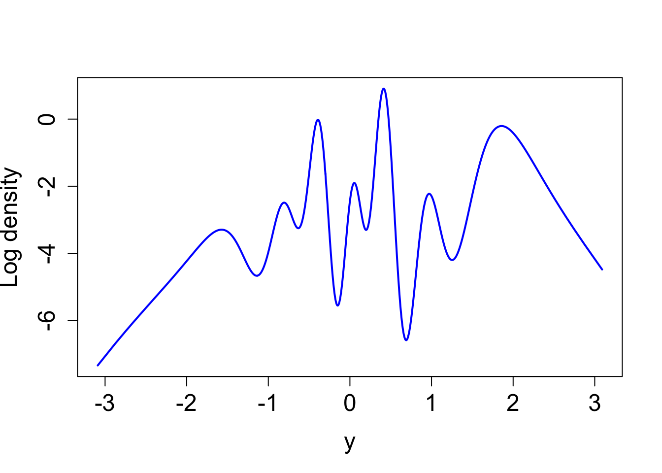
true_log_post <- function(x) {true_log_post_mapped(qnorm((x - lower)/(upper - lower))) - dnorm(qnorm((x - lower)/(upper - lower)), log = T) - log(upper - lower)}
integrate(function(x) exp(true_log_post(x)), lower = 0, upper = 10)
1 with absolute error < 9.1e-05plot(exp(true_log_post(x)) ~ x, type = "l", cex.lab = 1.5, cex.axis = 1.5,
xlab = "x", ylab = "Posterior density", lwd = 2, col = "blue")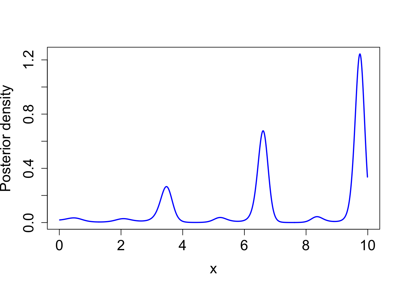
| Version | Author | Date |
|---|---|---|
| b5d1ce2 | Ziang Zhang | 2025-04-22 |
KL Divergence
Let \(f_t\) and \(f_{t-j}\) be the corresponding surrogate density at time \(t\) and \(t-j\), respectively. We can compute the KL divergence between \(f_t\) and \(f_{t-j}\) as follows: \[Q_t = KL(f_t,f_{t-j}) = \int \log \frac{f_t(x)}{f_{t-j}(x)}f_{t}(x)dx.\]
For one-dimensional problems, this can be done efficiently through numerical integration. For higher-dimensional problems, sampling-based methods can be used to approximate the KL divergence.
result_ad <- BOSS(
  func = eval_once, initial_design = 5,
  update_step = 5, max_iter = 30,
  opt.lengthscale.grid = 100, opt.grid = 1000,
  delta = 0.01, noise_var = noise_var,
  lower = lower, upper = upper,
  verbose = 0,
  KL_iter_check = 1, KL_check_warmup = 5, KL_eps = 0, criterion = "KL"
)

plot(result_ad$KL_result$KL ~ result_ad$KL_result$i,
     xlab = "Iteration", ylab = "KL statistic",
     main = "KL statistic over iterations",
     log = "y",
     pch = 19, col = "blue")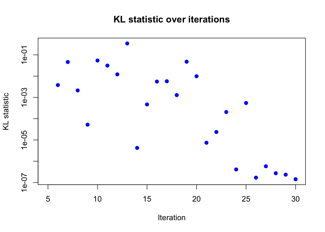
| Version | Author | Date |
|---|---|---|
| 6bb1cbf | Ziang Zhang | 2025-04-22 |
Based on the KL divergence, it seems like the algorithm has converged around 30 iterations.
KS Statistics
The Kolmogorov-Smirnov (KS) statistic measures the maximum difference between the cumulative distribution functions (CDFs) \(F_t\) and \(F_{t-j}\) of the surrogate densities \(f_t\) and \(f_{t-j}\), respectively. Specifically, for one dimensional problems, the KS statistic is defined as: \[Q_t = \max_x |F_t(x) - F_{t-j}(x)|.\]
result_ad <- BOSS(
  func = eval_once, initial_design = 5,
  update_step = 5, max_iter = 30,
  opt.lengthscale.grid = 100, opt.grid = 1000,
  delta = 0.01, noise_var = noise_var,
  lower = lower, upper = upper,
  verbose = 0,
  KS_iter_check = 1, KS_check_warmup = 5, KS_eps = 0, criterion = "KS"
)

plot(result_ad$KS_result$KS ~ result_ad$KS_result$i,
     xlab = "Iteration", ylab = "KS statistic",
     main = "KS statistic over iterations",
     log = "y",
     pch = 19, col = "blue")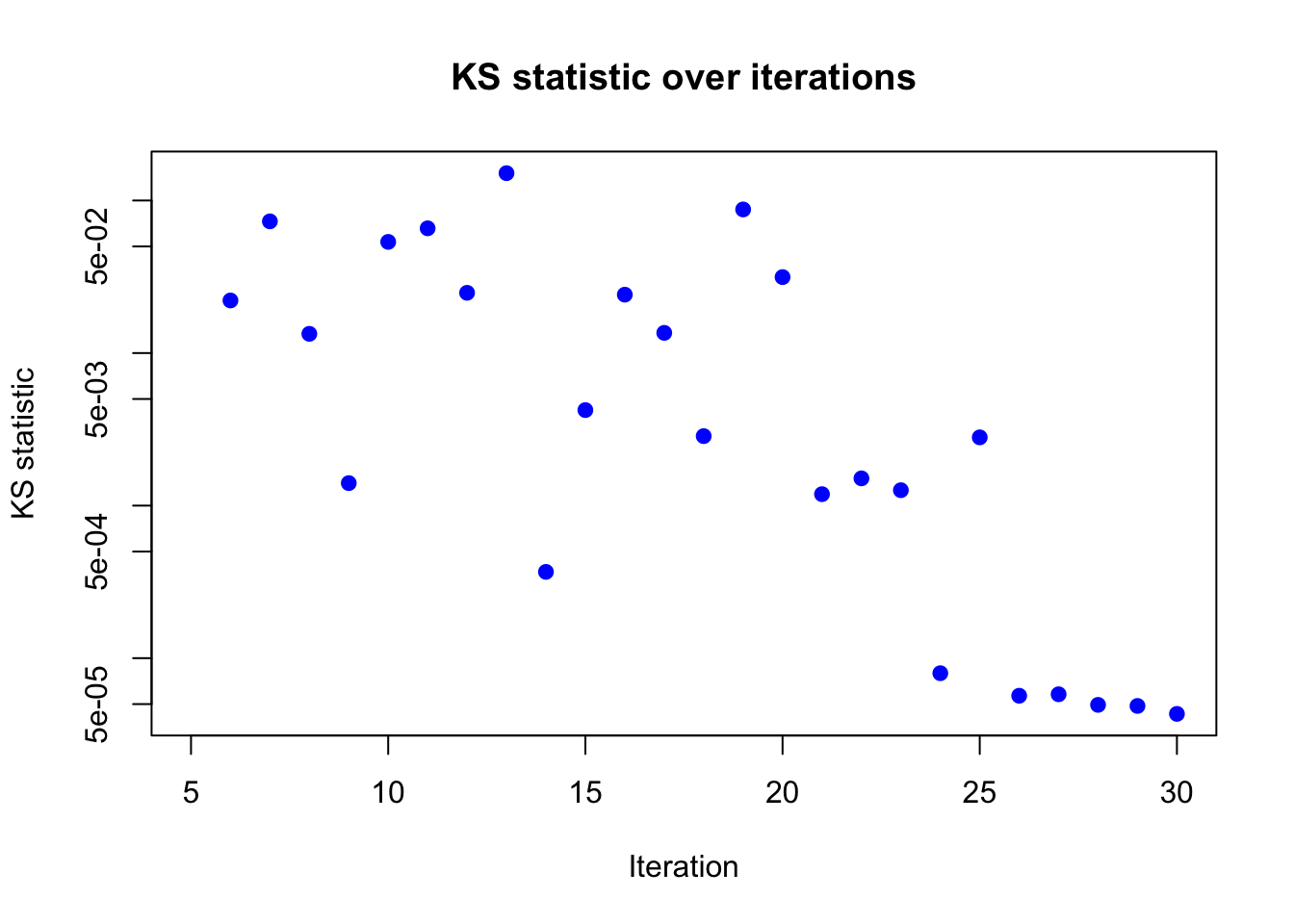
| Version | Author | Date |
|---|---|---|
| 6bb1cbf | Ziang Zhang | 2025-04-22 |
Based on the KS statistic, the conclusion is similar to that of the KL divergence. The KS statistics is very close to 0 after 30 iterations, indicating that the algorithm has likely converged.
Modal Convergence
For higher-dimensional problems, computing KL divergence is computationally more intensive due to the need for numerical integration or sampling-based methods.
Due to Bernstein-Von-Mises theorem, when the sample size is large, the majority of the posterior mass is concentrated around the mode. Thus, as an empirical heuristic, we can check the convergence of the modal behavior of the surrogate density. Although this method is less rigorous than KL divergence or KS statistic, it is computationally efficient and can be used as a quick diagnostic check for convergence.
For the modal behavior, we compute the average \(k\)-nearest neighbor distance between the current optimizer and its neighboring design points, as well as the relative change of the hessian (trace) at the current optimizer.
Specifically, define the current optimizer as \(\boldsymbol{\theta}_t^*\) and the average \(k\)-nearest neighbor distance of design points to \(\boldsymbol{\theta}_t^*\) as \(d_{t,k}\). Additionally, let \(H(\boldsymbol{\theta}_t^*)\) be the negative Hessian at \(\boldsymbol{\theta}_t^*\) based on the GP surrogate and write \(S_{t} = \sqrt{\mathrm{Tr}(H^{-1}(\boldsymbol{\theta}_t^*))}\). We can assess modal convergence by considering
- \(D_{t,k} = d_{t,k}/S_{t,k}\);
- \(H_{t} = \frac{S_{t} - S_{t-1}}{S_{t-1}}\).
We deem the algorithm to have reached convergence when \(Q_t =\max\{D_{t,k}, H_{t}\} < \varepsilon\) for some user-defined \(\varepsilon > 0\). Heuristically, \(S_{t}\) can be regarded as the size of the posterior standard deviation for sufficiently large \(t\). \(D_{t,k}\) thus gives a measure of how close the current optimizer is to the existing design points relative to the size of the posterior standard deviation. \(H_{t}\), on the other hand, gives a rough measure on the relative change of the size of the posterior standard deviation.
result_ad <- BOSS(
  func = eval_once, initial_design = 5,
  update_step = 5, max_iter = 30,
  opt.lengthscale.grid = 100, opt.grid = 1000,
  delta = 0.01, noise_var = noise_var,
  lower = lower, upper = upper,
  verbose = 0,
  modal_iter_check = 1, modal_check_warmup = 10, modal_k.nn = 5, modal_eps = 0, criterion = "modal"
)

plot(result_ad$modal_result$modal ~ result_ad$modal_result$i,
     xlab = "Iteration", ylab = "Modal statistic",
     main = "Modal statistic over iterations",
     log = "y",
     pch = 19, col = "blue")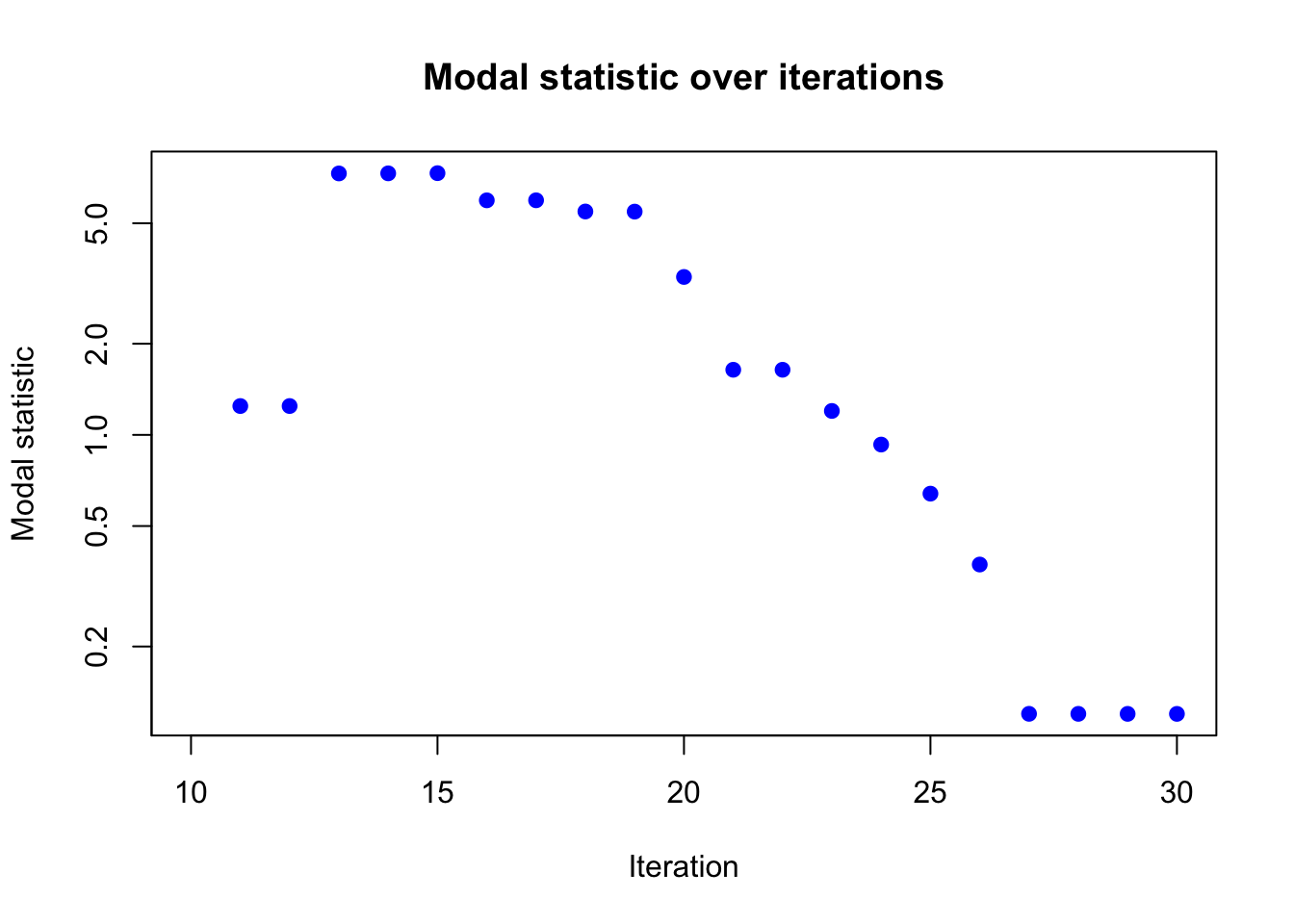
| Version | Author | Date |
|---|---|---|
| 6bb1cbf | Ziang Zhang | 2025-04-22 |
Again, the modal statistic converges to 0 after 30 iterations, indicating that the algorithm has likely converged.
sessionInfo()R version 4.3.1 (2023-06-16)
Platform: aarch64-apple-darwin20 (64-bit)
Running under: macOS Monterey 12.7.4
Matrix products: default
BLAS: /Library/Frameworks/R.framework/Versions/4.3-arm64/Resources/lib/libRblas.0.dylib
LAPACK: /Library/Frameworks/R.framework/Versions/4.3-arm64/Resources/lib/libRlapack.dylib; LAPACK version 3.11.0
locale:
[1] en_US.UTF-8/en_US.UTF-8/en_US.UTF-8/C/en_US.UTF-8/en_US.UTF-8
time zone: America/Chicago
tzcode source: internal
attached base packages:
[1] stats graphics grDevices utils datasets methods base
other attached packages:
[1] aghq_0.4.1 ggplot2_3.5.1 npreg_1.1.0 workflowr_1.7.1
loaded via a namespace (and not attached):
[1] sass_0.4.9 utf8_1.2.4 generics_0.1.3
[4] lattice_0.22-6 stringi_1.8.4 digest_0.6.37
[7] magrittr_2.0.3 evaluate_1.0.1 grid_4.3.1
[10] fastmap_1.2.0 rprojroot_2.0.4 jsonlite_1.8.9
[13] Matrix_1.6-4 processx_3.8.4 whisker_0.4.1
[16] ps_1.8.0 promises_1.3.0 httr_1.4.7
[19] fansi_1.0.6 scales_1.3.0 numDeriv_2016.8-1.1
[22] jquerylib_0.1.4 cli_3.6.3 rlang_1.1.4
[25] munsell_0.5.1 withr_3.0.2 cachem_1.1.0
[28] yaml_2.3.10 tools_4.3.1 dplyr_1.1.4
[31] colorspace_2.1-1 httpuv_1.6.15 vctrs_0.6.5
[34] R6_2.5.1 lifecycle_1.0.4 git2r_0.33.0
[37] stringr_1.5.1 fs_1.6.4 MASS_7.3-60
[40] pkgconfig_2.0.3 callr_3.7.6 pillar_1.9.0
[43] bslib_0.8.0 later_1.3.2 gtable_0.3.6
[46] glue_1.8.0 Rcpp_1.0.13-1 highr_0.11
[49] xfun_0.48 tibble_3.2.1 tidyselect_1.2.1
[52] rstudioapi_0.16.0 knitr_1.48 htmltools_0.5.8.1
[55] rmarkdown_2.28 compiler_4.3.1 getPass_0.2-4